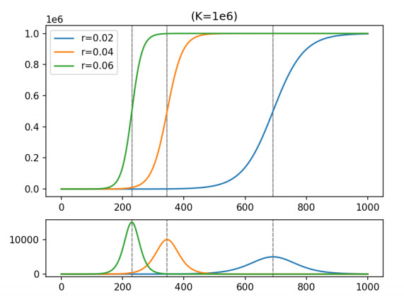
Accurately estimating the number of infections that actually occur in the earliest phases of an outbreak and predicting the number of new cases per day in various countries is crucial for real-time monitoring of COVID-19 transmission. Numerous studies have used mathematical models to predict the progression of infection rates in several countries following the appearance of epidemiological outbreaks. In this study, we analyze the data reported and then study several logistical-type phenomenological models and their application in practice for forecasting infection evolution. When several epidemic waves follow one another, it is important to stress that a traditional logistic model cannot necessarily be fully adapted to the data made available. New models are being introduced to simultaneously take account of human behavior, measures taken by the government, and epidemiological conditions. This research used a generalized logistic model based on parameters that vary over time to describe trends in COVID-19-infected cases in countries that have undergone several waves. In two-wave scenarios, the parameters of the model evolve dynamically over time following a logistic function, where the first and second waves are characterized by two extreme values for the early period and the late one, respectively.
Citation: Said Gounane, Jamal Bakkas, Mohamed Hanine, Gyu Sang Choi, Imran Ashraf. Generalized logistic model with time-varying parameters to analyze COVID-19 outbreak data[J]. AIMS Mathematics, 2024, 9(7): 18589-18607. doi: 10.3934/math.2024905
Accurately estimating the number of infections that actually occur in the earliest phases of an outbreak and predicting the number of new cases per day in various countries is crucial for real-time monitoring of COVID-19 transmission. Numerous studies have used mathematical models to predict the progression of infection rates in several countries following the appearance of epidemiological outbreaks. In this study, we analyze the data reported and then study several logistical-type phenomenological models and their application in practice for forecasting infection evolution. When several epidemic waves follow one another, it is important to stress that a traditional logistic model cannot necessarily be fully adapted to the data made available. New models are being introduced to simultaneously take account of human behavior, measures taken by the government, and epidemiological conditions. This research used a generalized logistic model based on parameters that vary over time to describe trends in COVID-19-infected cases in countries that have undergone several waves. In two-wave scenarios, the parameters of the model evolve dynamically over time following a logistic function, where the first and second waves are characterized by two extreme values for the early period and the late one, respectively.

| [1] | G. Chowell, Fitting dynamic models to epidemic outbreaks with quantified uncertainty: A primer for parameter uncertainty, identifiability, and forecasts, Infect. Dis. Modell., 2 (2017), 379–398. |
| [2] |
H. Heesterbeek, R. M. Anderson, V. Andreasen, S. Bansal, D. De Angelis, C. Dye, et al., Modeling infectious disease dynamics in the complex landscape of global health, Science, 347 (2015), aaa4339. https://doi.org/10.1126/science.aaa4339 doi: 10.1126/science.aaa4339

|
| [3] | S. Funk, M. Salathe, V. A. A. Jansen, Modelling the influence of human behaviour on the spread of infectious diseases: A review, J. Royal Soc., Interface, 7 (2010), 1247–1256. |
| [4] | C. Poletto, M. Gomes, Y. P. A. Pastore, L. Rossi, L. Bioglio, D. Chao, et al., Assessing the impact of travel restrictions on international spread of the 2014 West African Ebola epidemic, Eurosurveillance, 19 (2014). |
| [5] | D. Okuonghae, A. Omame, Analysis of a mathematical model for COVID-19 population dynamics in Lagos, Nigeria, Chaos, Solution. Fract., 139 (2020), 110032. |
| [6] |
A. Omame, D. Okuonghae, U. K. Nwajeri, C. P. Onyenegecha, A fractional-order multi-vaccination model for COVID-19 with non-singular kernel, Alexandria Eng. J., 61 (2022), 6089–6104. https://doi.org/10.1016/j.aej.2021.11.037 doi: 10.1016/j.aej.2021.11.037
|
| [7] | S. F. Verhulst, Notice sur la loi que la population suit dans son accroissement. Corr. Math.Physics. 10 (1838) 113. |
| [8] |
H. Ghosh, M. A. Iquebal, Prajneshu, Bootstrap study of parameter estimates for nonlinear Richards growth model through genetic algorithm, J. Appl. Stat., 38 (2011), 491–500. https://doi.org/10.1080/02664760903521401 doi: 10.1080/02664760903521401
|
| [9] |
J. Lv, K. Wang, J. Jiao, Stability of stochastic Richards growth model, Appl. Math. Modell., 39 (2015), 4821–4827. https://doi.org/10.1016/j.apm.2015.04.016 doi: 10.1016/j.apm.2015.04.016
|
| [10] |
X. Wang, J. Wu, Y. Yang, Richards model revisited: Validation by and application to infection dynamics, J. Theor. Biol., 313 (2012), 12–19. https://doi.org/10.1016/j.jtbi.2012.07.024 doi: 10.1016/j.jtbi.2012.07.024
|
| [11] | G. Himadri, Prajneshu, Optimum Fitting of Richards Growth Model in Random Environment, J. Stat. Theory Pract., 13 (2019), 6. |
| [12] |
P. Meyer, Bi-logistic growth, Technol. Forecast. Soc. Change, 47 (1994), 89–102. https://doi.org/10.1016/0040-1625(94)90042-6 doi: 10.1016/0040-1625(94)90042-6
|
| [13] | S. Gounane, J. Bakkas, F. Karami, Y. Barkouch, Nonlinear Growth Models with Lockdown Periods for Analyzing Cumulative and Daily COVID-19 Outbreak Data, IEEE International Conference on Advances in Data-Driven Analytics And Intelligent Systems (ADACIS), 2023, 1–6. http://doi.org/10.1109/ADACIS59737.2023.10424370 |
| [14] | GitHub, Covid-19 repository at github, 2020. Available from: https://github.com/CSSEGISandData/COVID-19. |
| [15] |
E. Dong, H. Du, L. Gardner, An interactive web-based dashboard to track COVID-19 in real time, Lancet Infect. Dis., 20 (2020), 533–534. https://doi.org/10.1016/S1473-3099(20)30120-1 doi: 10.1016/S1473-3099(20)30120-1
|
| [16] | E. Dong, J. Ratcliff, T. D. Goyea, A. Katz, R. Lau, T. K. Ng, et al., The Johns Hopkins University Center for Systems Science and Engineering COVID-19 Dashboard: Data collection process, challenges faced, and lessons learned, Lancet. Infect. Dis., 22 (2022), e370–e376. https://doi.org/10.1016/S1473-3099(22)00434-0 |
| [17] | H. T. Banks, S. Hu, W. C. Thompson, Modeling and inverse problems in the presence of uncertainty, New York: Chapman and Hall/CRC, 2014. |


Figures(8)

Said Gounane, Jamal Bakkas, Mohamed Hanine, Gyu Sang Choi, Imran Ashraf. Generalized logistic model with time-varying parameters to analyze COVID-19 outbreak data[J]. AIMS Mathematics, 2024, 9(7): 18589-18607. doi: 10.3934/math.2024905


 DownLoad: