q-Rung Orthopair fuzzy time series forecasting technique: Prediction based decision making

Shahzaib Ashraf; Muhammad Shakir Chohan; Sameh Askar; Noman Jabbar; Shahzaib Ashraf; Muhammad Shakir Chohan; Sameh Askar; Noman Jabbar

doi:10.3934/math.2024272

AIMS Mathematics

2024, Volume 9, Issue 3: 5633-5660. doi: 10.3934/math.2024272

Previous Article Next Article

Research article Special Issues

q-Rung Orthopair fuzzy time series forecasting technique: Prediction based decision making

1.
Institute of Mathematics, Khwaja Fareed University of Engineering and Information Technology, Rahim Yar Khan 64200, Pakistan
2.
Department of Statistics and Operations Research, College of Science, King Saud University, P.O. Box 2455, Riyadh 11451, Saudi Arabia
3.
Institute of Structure Analysis, Poznan University of Technology, 61-138 Poznan, Poland

Received: 20 March 2023 Revised: 26 June 2023 Accepted: 11 July 2023 Published: 30 January 2024

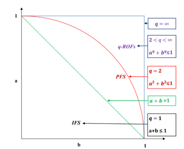
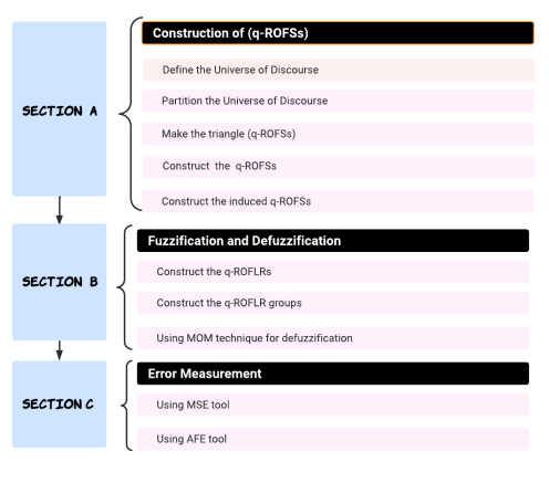
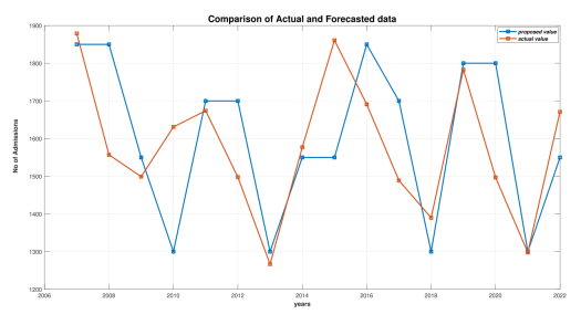
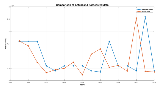
The literature frequently uses fuzzy inference methods for time series forecasting. In business and other situations, it is frequently necessary to forecast numerous time series. The q-Rung orthopair fuzzy set is a beneficial and competent tool to address ambiguity. In this research, a computational forecasting method based on q-Rung orthopair fuzzy time series has been created to deliver better prediction results to deal with situations containing higher uncertainty caused by large fluctuations in consecutive years' values in time series data and with no visualization of trend or periodicity. The main objective of this article is to handle time series forecasting with the usage of q-Rung orthopair fuzzy sets for things like floods, admission of students, number of patients, etc. After this, people can then manage issues that will arise in the future. Previously, there was a gap in determining the forecasting of data whose entire value of membership and non-membership exceeded 1. To fill this kind of gap, we used q-Rung orthopair fuzzy sets in time series forecasting. We also used numerous algebraic components for the q-Rung orthopair fuzzy time series, which has a union, max-min composition, cartesian product, and algorithm that are useful to calculate the method of data forecasting. Moreover, we also defined the algorithm and proposed MATLAB code that facilitates the execution of mathematical calculations, design, analysis, and optimization (structural and mathematical), and gives results with speed, correctness, and precision. At the end, we tested the model using historical student enrollment data and the annual peak discharge at Guddu Barrage. Furthermore, we calculated the error to get an idea of to what extent this method is suitable.
- fuzzy time series,
- intuitionistic fuzzy sets,
- q-Rung orthopair fuzzy sets,
- induced fuzzy set,
- nondeterminacy
Citation: Shahzaib Ashraf, Muhammad Shakir Chohan, Sameh Askar, Noman Jabbar. q-Rung Orthopair fuzzy time series forecasting technique: Prediction based decision making[J]. AIMS Mathematics, 2024, 9(3): 5633-5660. doi: 10.3934/math.2024272

Related Papers:

Abstract

The literature frequently uses fuzzy inference methods for time series forecasting. In business and other situations, it is frequently necessary to forecast numerous time series. The q-Rung orthopair fuzzy set is a beneficial and competent tool to address ambiguity. In this research, a computational forecasting method based on q-Rung orthopair fuzzy time series has been created to deliver better prediction results to deal with situations containing higher uncertainty caused by large fluctuations in consecutive years' values in time series data and with no visualization of trend or periodicity. The main objective of this article is to handle time series forecasting with the usage of q-Rung orthopair fuzzy sets for things like floods, admission of students, number of patients, etc. After this, people can then manage issues that will arise in the future. Previously, there was a gap in determining the forecasting of data whose entire value of membership and non-membership exceeded 1. To fill this kind of gap, we used q-Rung orthopair fuzzy sets in time series forecasting. We also used numerous algebraic components for the q-Rung orthopair fuzzy time series, which has a union, max-min composition, cartesian product, and algorithm that are useful to calculate the method of data forecasting. Moreover, we also defined the algorithm and proposed MATLAB code that facilitates the execution of mathematical calculations, design, analysis, and optimization (structural and mathematical), and gives results with speed, correctness, and precision. At the end, we tested the model using historical student enrollment data and the annual peak discharge at Guddu Barrage. Furthermore, we calculated the error to get an idea of to what extent this method is suitable.

References

[1]	S. Ashraf, M. S. Chohan, S. Ahmad, M. S. Hameed, F. Khan, Decision Aid Algorithm for Kidney Transplants Under Disc Spherical Fuzzy Sets With Distinctive Radii Information, IEEE Access, 11 (2023), 122029–122044. https://doi.org/10.1109/ACCESS.2023.3327830 doi: 10.1109/ACCESS.2023.3327830
[2]	F. A. Lootsma, Fuzzy logic for planning and decision making, New York: Springer, 2013.
[3]	L. Zadeh, Fuzzy sets, In: Fuzzy sets, fuzzy logic, and fuzzy systems, New York: World Scientific, 1996,394–432. http://dx.doi.org/10.1142/9789814261302_0021
[4]	K. T. Atanassov, On intuitionistic fuzzy sets theory, Berlin, Heidelberg: Springer, 2012.
[5]	K. T. Atanassov, More on intuitionistic fuzzy sets, Fuzzy sets Syst., 33 (1989), 37–45. https://doi.org/10.1007/978-3-642-10646-028 doi: 10.1007/978-3-642-10646-028
[6]	D. J. Dubois, Fuzzy sets and systems: Theory and applications, Orlando: Academic Press, 1980.
[7]	N. Cagman, S. Enginoglu, F. Citak, Fuzzy soft set theory and its applications, Iran. J. Fuzzy Syst., 8 (2011), 137–147.
[8]	N. Cagman, S. Karatas, Intuitionistic fuzzy soft set theory and its decision making, J. Intell. Fuzzy Syst., 2 (2013), 829–836. https://doi.org/10.3233/IFS-2012-0601 doi: 10.3233/IFS-2012-0601
[9]	L. Lin, X. H. Yuan, Z. Q. Xia, Multicriteria fuzzy decision-making methods based on intuitionistic fuzzy sets, J. Comput. Syst. Sci., 73 (2007), 84–88. https://doi.org/10.1016/j.jcss.2006.03.004 doi: 10.1016/j.jcss.2006.03.004
[10]	J. Q. Wang, R. R. Nie, H. Y. Zhang, X. H. Chen, Intuitionistic fuzzy multi-criteria decision-making method based on evidential reasoning, Appl. Soft Comput., 13 (2013), 1823–1831. https://doi.org/10.1016/j.asoc.2012.12.019 doi: 10.1016/j.asoc.2012.12.019
[11]	Q. Song, B. S. Chissom, Fuzzy time series and its models, Fuzzy Sets Syst., 54 (1993), 269–277. https://doi.org/10.1016/0165-0114(93)90372-O doi: 10.1016/0165-0114(93)90372-O
[12]	Q. Song, B. S. Chissom, Forecasting enrollments with fuzzy time series Part Ⅰ, Fuzzy Sets Syst., 54 (1993), 1–9. https://doi.org/10.1016/0165-0114(93)90355-L doi: 10.1016/0165-0114(93)90355-L
[13]	Q. Song, B. S. Chissom, Forecasting enrollments with fuzzy time series Part Ⅱ, Fuzzy Sets Syst., 62 (1994), 1–8. https://doi.org/10.1016/0165-0114(94)90067-1 doi: 10.1016/0165-0114(94)90067-1
[14]	S. Kumar, S. S Gangwar, Intuitionistic fuzzy time series: An approach for handling nondeterminism in time series forecasting, IEEE Trans. Fuzzy Syst., 24 (2015), 1270–1281. https://doi.org/10.1109/TFUZZ.2015.2507582 doi: 10.1109/TFUZZ.2015.2507582
[15]	B. P. Joshi, S. Kumar, A computational method of forecasting based on intuitionistic fuzzy sets and fuzzy time series, Proceedings of the International Conference on Soft Computing for Problem Solving (SocProS 2011) December 20-22, 2011, 2012,993–1000. https://doi.org/10.1007/978-81-322-0491-691
[16]	B. P. Joshi, S. Kumar, Intuitionistic fuzzy sets based method for fuzzy time series forecasting, Cybern. Syst., 43 (2012), 34–47. https://doi.org/10.1080/01969722.2012.637014 doi: 10.1080/01969722.2012.637014
[17]	S. S. Gangwar, S. Kumar, Probabilistic and intuitionistic fuzzy sets based method for fuzzy time series forecasting, Cybern. Syst., 45 (2014), 349–361. https://doi.org/10.1080/01969722.2014.904135 doi: 10.1080/01969722.2014.904135
[18]	C. H. Cheng, G. W. Cheng, J. W. Wang, Multi-attribute fuzzy time series method based on fuzzy clustering, Expert Syst. Appl., 34 (2008), 1235–1242. https://doi.org/10.1016/j.eswa.2006.12.013 doi: 10.1016/j.eswa.2006.12.013
[19]	M. T. Chou, Long-term predictive value interval with the fuzzy time series, J. Mar. Sci. Technol., 19 (2011), 6. https://doi.org/10.51400/2709-6998.2164 doi: 10.51400/2709-6998.2164
[20]	R. R. Yager, Generalized orthopair fuzzy sets, IEEE Trans. Fuzzy Syst., 25 (2016), 1222–1230. https://doi.org/10.1109/TFUZZ.2016.2604005 doi: 10.1109/TFUZZ.2016.2604005
[21]	R. R. Yager, N. Alajlan, Approximate reasoning with generalized orthopair fuzzy sets, Inf. Fusion, 38 (2017), 65–73. https://doi.org/10.1016/j.inffus.2017.02.005 doi: 10.1016/j.inffus.2017.02.005
[22]	R. R. Yager, A. M. Abbasov, Pythagorean membership grades, complex numbers, and decision making, Int. J. Intell. Syst., 28 (2013), 436–452. https://doi.org/10.1002/int.21584 doi: 10.1002/int.21584
[23]	R. R Yager, Pythagorean fuzzy subsets, 2013 joint IFSA world congress and NAFIPS annual meeting (IFSA/NAFIPS), 2013, 57–61. https://doi.org/10.1109/IFSA-NAFIPS.2013.6608375
[24]	A. B. Khoshaim, S. Abdullah, S. Ashraf, M. Naeem, Emergency decision-making based on q-rung orthopair fuzzy rough aggregation information, CMC, 69 (2021), 4077–4094. https://doi.org/10.32604/cmc.2021.016973 doi: 10.32604/cmc.2021.016973
[25]	T. Shaheen, M. T. Ali, H. Toor, Why do we need q-rung orthopair fuzzy sets? Some evidence established via mass assignment, Int. J. Intell. Syst., 36 (2021), 5493–5505. https://doi.org/10.1002/int.22520 doi: 10.1002/int.22520
[26]	S. Ashraf, N. Rehman, A. Hussain, H. AlSalman, A. H. Gumaei, q-Rung Orthopair Fuzzy Rough Einstein Aggregation Information-Based EDAS Method: Applications in Robotic Agrifarming, Comput. Intell. Neurosci., 2021 (2021), 5520264. https://doi.org/10.1155/2021/5520264 doi: 10.1155/2021/5520264
[27]	P. Liu, Y. Li, P. Wang, Consistency threshold-and score function-based multi-attribute decision-making with Q-rung orthopair fuzzy preference relations, Inf. Sci., 618 (2022), 356–378. https://doi.org/10.1016/j.ins.2022.10.122 doi: 10.1016/j.ins.2022.10.122
[28]	H. Garg, K. Ullah, T. Mahmood, N. Hassan, N. Jan, T-spherical fuzzy power aggregation operators and their applications in multi-attribute decision making, J. Ambient. Intell. Human. Comput., 12 (2021), 9067–9080. https://doi.org/10.1007/s12652-020-02600-z doi: 10.1007/s12652-020-02600-z
[29]	P. Liu, Q. Khan, T. Mahmood, N. Hassan, T-spherical fuzzy power Muirhead mean operator based on novel operational laws and their application in multi-attribute group decision making, IEEE Access, 7 (2019), 22613–22632. https://doi.org/10.1109/ACCESS.2019.2896107 doi: 10.1109/ACCESS.2019.2896107
[30]	A. Khan, S. S. Abosuliman, S. Ashraf, S. Abdullah, Hospital admission and care of COVID-19 patients problem based on spherical hesitant fuzzy decision support system, Int. J. Intell. Syst., 36 (2021), 4167–4209. https://doi.org/10.1002/int.22455 doi: 10.1002/int.22455
[31]	S. M. Chen, Forecasting enrollments based on fuzzy time series, Fuzzy Sets Syst., 81 (1996), 311–319. https://doi.org/10.1016/0165-0114(95)00220-0 doi: 10.1016/0165-0114(95)00220-0
[32]	B. P. Joshi, S. Kumar, Intuitionistic fuzzy sets based method for fuzzy time series forecasting, Cybern. Syst., 43 (2012), 34–47. https://doi.org/10.1080/01969722.2012.637014 doi: 10.1080/01969722.2012.637014
[33]	S. Kumar, S. S. Gangwar, A fuzzy time series forecasting method induced by intuitionistic fuzzy sets, Int. J. Model., Simul., Sci. Comput., 6 (2015), 1550041. https://doi.org/10.1142/S1793962315500415 doi: 10.1142/S1793962315500415
[34]	S. S. Gautam, S. R. Singh, A refined method of forecasting based on high-order intuitionistic fuzzy time series data, Prog. Artif. Intell., 7 (2018), 339–350. https://doi.org/10.1007/s13748-018-0152-x doi: 10.1007/s13748-018-0152-x
[35]	P. Wang, J. Wang, G. Wei, C. Wei, Similarity measures of q-rung orthopair fuzzy sets based on cosine function and their applications, Mathematics, 7 (2019), 340. https://doi.org/10.3390/math7040340 doi: 10.3390/math7040340
[36]	M. H. Azam, M. H. Hasan, S. Hassan, S. J. Abdulkadir, Fuzzy type-1 triangular membership function approximation using fuzzy C-means, 2020 International Conferenceon Computational Intelligence (ICCI), (2020), 115–120. https://doi.org/10.1109/ICCI51257.2020.9247773
[37]	S. R. Singh, A simple time variant method for fuzzy time series forecasting, Cybern. Syst.:Int. J., 38 (2007), 305–321. https://doi.org/10.1080/01969720601187354 doi: 10.1080/01969720601187354
[38]	A. Jurio, D. Paternain, H. Bustince, C. Guerra, G. Beliakov, A construction method of Atanassov's intuitionistic fuzzy sets for image processing, 2010 5th IEEE International Conference Intelligent Systems, (2010), 337–342. https://doi.org/10.1109/IS.2010.5548390
[39]	U. Yolcu, E. Egrioglu, V. R. Uslu, M. A. Ba saran, C. H. Aladag, A new approach for determining the length of intervals for fuzzy time series, Appl. Soft Comput., 9 (2009), 647–651. https://doi.org/10.1016/j.asoc.2008.09.002 doi: 10.1016/j.asoc.2008.09.002

Reader Comments

Your name:*

Email:*
© 2024 the Author(s), licensee AIMS Press. This is an open access article distributed under the terms of the Creative Commons Attribution License (http://creativecommons.org/licenses/by/4.0)