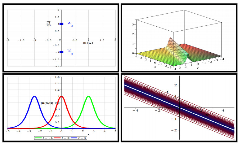
Our objective is to explore the intricacies of a nonlinear nonlocal fifth-order scalar Sasa-Satsuma equation in reverse spacetime which is rooted in a nonlocal $ 5 \times 5 $ matrix AKNS spectral problem. Starting with this spectral problem, we derive both local and nonlocal symmetry relations through rotations within a defined group. We then formulate a specific type of Riemann-Hilbert problem, facilitating the generation of soliton solutions. These solutions are generated by utilizing vectors that reside in the kernel of the matrix Jost solutions. Under the condition where reflection coefficients are null, the jump matrix reduces to the identity, leading to soliton solutions via the corresponding Riemann-Hilbert problem. The explicit formulas of these soliton solutions enable a comprehensive exploration of their dynamics.
Citation: Ahmed M. G. Ahmed, Alle Adjiri, Solomon Manukure. Soliton solutions and a bi-Hamiltonian structure of the fifth-order nonlocal reverse-spacetime Sasa-Satsuma-type hierarchy via the Riemann-Hilbert approach[J]. AIMS Mathematics, 2024, 9(9): 23234-23267. doi: 10.3934/math.20241130
Our objective is to explore the intricacies of a nonlinear nonlocal fifth-order scalar Sasa-Satsuma equation in reverse spacetime which is rooted in a nonlocal $ 5 \times 5 $ matrix AKNS spectral problem. Starting with this spectral problem, we derive both local and nonlocal symmetry relations through rotations within a defined group. We then formulate a specific type of Riemann-Hilbert problem, facilitating the generation of soliton solutions. These solutions are generated by utilizing vectors that reside in the kernel of the matrix Jost solutions. Under the condition where reflection coefficients are null, the jump matrix reduces to the identity, leading to soliton solutions via the corresponding Riemann-Hilbert problem. The explicit formulas of these soliton solutions enable a comprehensive exploration of their dynamics.

| [1] |
Z. Z. Kang, T. C. Xia, Construction of multi-soliton solutions of the $N$-coupled Hirota equations in an optical fiber, Chinese Phys. Lett., 36 (2019), 110201. https://doi.org/10.1088/0256-307X/36/11/110201 doi: 10.1088/0256-307X/36/11/110201

|
| [2] | A. R. Osborne, Nonlinear ocean waves and the inverse scattering transform, Academic Press, 2010. |
| [3] |
M. J. Ablowitz, Z. H. Musslimani, Inverse scattering transform for the integrable nonlocal nonlinear Schrödinger equation, Nonlinearity, 29 (2016), 915. https://doi.org/10.1088/0951-7715/29/3/915 doi: 10.1088/0951-7715/29/3/915
|
| [4] |
M. J. Ablowitz, D. J. Kaup, A. C. Newell, H. Segur, The inverse scattering transform-Fourier analysis for nonlinear problems, Stud. Appl. Math., 53 (1974), 249–315. https://doi.org/10.1002/sapm1974534249 doi: 10.1002/sapm1974534249
|
| [5] | M. J. Ablowitz, P. A. Clarkson, Solitons, nonlinear evolution equations and inverse scattering, Cambridge University Press, 1991. |
| [6] | M. J. Ablowitz, H. Segur, Solitons and the inverse scattering transform, Philadelphia: SIAM, 1981. |
| [7] |
W. X. Ma, Y. H. Huang, F. D. Wang, Inverse scattering transforms and soliton solutions of nonlocal reverse-space nonlinear Schrodinger hierarchies, Stud. Appl. Math., 145 (2020), 563–585. https://doi.org/10.1111/sapm.12329 doi: 10.1111/sapm.12329
|
| [8] |
L. M. Ling, W. X. Ma, Inverse scattering and soliton solutions of nonlocal complex reverse-spacetime modified Korteweg-de Vries hierarchies, Symmetry, 13 (2021), 1–17. https://doi.org/10.3390/sym13030512 doi: 10.3390/sym13030512
|
| [9] | J. Yang, Physically significant nonlocal nonlinear Schrödinger equation and its soliton solutions, Phys. Rev. E, 98 (2018), 042202. |
| [10] | M. J. Ablowitz, A. S. Fokas, Complex variables: introduction and applications, Cambridge University Press, 2003. |
| [11] |
W. X. Ma, Nonlocal PT-symmetric integrable equations and related Riemann-Hilbert problems, Partial Differ. Equ. Appl. Math., 4 (2021), 100190. https://doi.org/10.1016/j.padiff.2021.100190 doi: 10.1016/j.padiff.2021.100190
|
| [12] |
X. G. Geng, M. M. Chen, K. D. Wang, Application of the nonlinear steepest descent method to the coupled Sasa-Satsuma equation, East Asian J. Appl. Math., 11 (2021), 181–206. https://doi.org/10.4208/eajam.220920.250920 doi: 10.4208/eajam.220920.250920
|
| [13] |
Y. H. Li, R. M. Li, B. Xue, X. G. Geng, A generalized complex mKdV equation: Darboux transformations and explicit solutions, Wave Motion, 98 (2020), 102639. https://doi.org/10.1016/j.wavemoti.2020.102639 doi: 10.1016/j.wavemoti.2020.102639
|
| [14] |
Z. K. Kang, T. C. Xia, W. X. Ma, Riemann-Hilbert approach and $N$-soliton solution for an eighth-order nonlinear Schrödinger equation in an optical fiber, Adv. Differ. Equ., 2019 (2019), 1–14. https://doi.org/10.1186/s13662-019-2121-5 doi: 10.1186/s13662-019-2121-5
|
| [15] |
W. X. Ma, Riemann-Hilbert problems of a six-component fourth-order AKNS system and its soliton solutions, Comput. Appl. Math., 37 (2018), 6359–6375. https://doi.org/10.1007/s40314-018-0703-6 doi: 10.1007/s40314-018-0703-6
|
| [16] |
W. X. Ma, Riemann-Hilbert problems and soliton solutions of a multicomponent mKdV system and its reduction, Math. Methods Appl. Sci., 42 (2019), 1099–1113. https://doi.org/10.1002/mma.5416 doi: 10.1002/mma.5416
|
| [17] |
W. X. Ma, Y. Zhou, Reduced D-Kaup-Newell soliton hierarchies from sl(2, $\mathbb{R}$) and so(3, $\mathbb{R}$), Int. J. Geom. Methods Modern Phys., 13 (2016), 1650105. https://doi.org/10.1142/S021988781650105X doi: 10.1142/S021988781650105X
|
| [18] |
W. X. Ma, Inverse scattering for nonlocal reverse-time nonlinear Schrödinger equations, Appl. Math. Lett., 102 (2020), 106161. https://doi.org/10.1016/j.aml.2019.106161 doi: 10.1016/j.aml.2019.106161
|
| [19] |
W. X. Ma, Riemann-Hilbert problems and $N$-soliton solutions for a coupled mKdV system, J. Geom. Phys., 132 (2018), 45–54. https://doi.org/10.1016/j.geomphys.2018.05.024 doi: 10.1016/j.geomphys.2018.05.024
|
| [20] |
W. X. Ma, Riemann-Hilbert problems and soliton solutions of type $(\lambda^{*}, -\lambda^{*})$ reduced nonlocal integrable mKdV hierarchies, Mathematics, 10 (2022), 1–21. https://doi.org/10.3390/math10060870 doi: 10.3390/math10060870
|
| [21] |
W. X. Ma, Riemann-Hilbert problems and soliton solutions of nonlocal reverse-time NLS hierarchies, Acta Math. Sci., 42 (2022), 127–140. https://doi.org/10.1007/s10473-022-0106-z doi: 10.1007/s10473-022-0106-z
|
| [22] | J. Yang, Nonlinear waves in integrable and non-integrable systems, Philadelphia: SIAM, 2010. |
| [23] | T. Trogdon, S. Olver, Riemann-Hilbert problems, their numerical solution, and the computation of nonlinear special functions, Philadelphia: SIAM, 2015. |
| [24] | P. G. Drazin, R. S. Johnson, Solitons: an introduction, Cambridge University Press, 1989. |
| [25] | W. X. Ma, Inverse scattering and soliton solutions of nonlocal reverse-spacetime nonlinear Schrödinger equations, Proc. Amer. Math. Soc., 149 (2021), 251–263. |
| [26] |
J. K. Yang, General $N$-solitons and their dynamics in several nonlinear Schrödinger equations, Phys. Lett. A, 383 (2019), 328–337. https://doi.org/10.1016/j.physleta.2018.10.051 doi: 10.1016/j.physleta.2018.10.051
|
| [27] |
A. Adjiri, A. M. G. Ahmed, W. X. Ma, Riemann-Hilbert problems of a nonlocal reverse-time six-component AKNS system of fourth order and its exact soliton solutions, Int. J. Modern Phys. B, 35 (2021), 2150035. https://doi.org/10.1142/S0217979221500351 doi: 10.1142/S0217979221500351
|
| [28] | V. B. Matveev, M. A. Salle, Darboux transformations and solitons, Springer, 1991. |
| [29] | R. Hirota, The direct method in soliton theory, Cambridge University Press, 2004. |
| [30] |
Y. L. Sun, W. X. Ma, J. P. Yu, $N$-soliton solutions and dynamic property analysis of a generalized three-component Hirota-Satsuma coupled KdV equation, Appl. Math. Lett., 120 (2021), 107224. https://doi.org/10.1016/j.aml.2021.107224 doi: 10.1016/j.aml.2021.107224
|


Figures(9)

Ahmed M. G. Ahmed, Alle Adjiri, Solomon Manukure. Soliton solutions and a bi-Hamiltonian structure of the fifth-order nonlocal reverse-spacetime Sasa-Satsuma-type hierarchy via the Riemann-Hilbert approach[J]. AIMS Mathematics, 2024, 9(9): 23234-23267. doi: 10.3934/math.20241130


 DownLoad: