Control and elimination in an SEIR model for the disease dynamics of COVID-19 with vaccination

Peter Joseph Witbooi; Sibaliwe Maku Vyambwera; Mozart Umba Nsuami; Peter Joseph Witbooi; Sibaliwe Maku Vyambwera; Mozart Umba Nsuami

doi:10.3934/math.2023411

AIMS Mathematics

2023, Volume 8, Issue 4: 8144-8161. doi: 10.3934/math.2023411

Previous Article Next Article

Research article

Control and elimination in an SEIR model for the disease dynamics of COVID-19 with vaccination

Department of Mathematics and Applied Mathematics, University of the Western Cape, Private Bag X17, Bellville 7535, Republic of South Africa

Received: 04 September 2022 Revised: 16 November 2022 Accepted: 22 November 2022 Published: 31 January 2023
MSC : 92D30, 34K20

COVID-19 has become a serious pandemic affecting many countries around the world since it was discovered in 2019. In this research, we present a compartmental model in ordinary differential equations for COVID-19 with vaccination, inflow of infected and a generalized contact rate. Existence of a unique global positive solution of the model is proved, followed by stability analysis of the equilibrium points. A control problem is presented, with vaccination as well as reduction of the contact rate by way of education, law enforcement or lockdown. In the last section, we use numerical simulations with data applicable to South Africa, for supporting our theoretical results. The model and application illustrate the interesting manner in which a diseased population can be perturbed from within itself.
- basic reproduction number,
- generalized contact rate,
- infected immigrants,
- awareness,
- alertness
Citation: Peter Joseph Witbooi, Sibaliwe Maku Vyambwera, Mozart Umba Nsuami. Control and elimination in an SEIR model for the disease dynamics of COVID-19 with vaccination[J]. AIMS Mathematics, 2023, 8(4): 8144-8161. doi: 10.3934/math.2023411

Related Papers:

Abstract

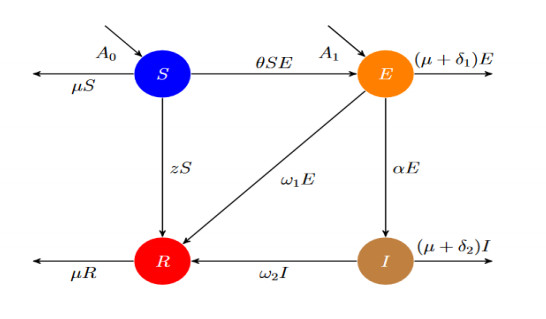
COVID-19 has become a serious pandemic affecting many countries around the world since it was discovered in 2019. In this research, we present a compartmental model in ordinary differential equations for COVID-19 with vaccination, inflow of infected and a generalized contact rate. Existence of a unique global positive solution of the model is proved, followed by stability analysis of the equilibrium points. A control problem is presented, with vaccination as well as reduction of the contact rate by way of education, law enforcement or lockdown. In the last section, we use numerical simulations with data applicable to South Africa, for supporting our theoretical results. The model and application illustrate the interesting manner in which a diseased population can be perturbed from within itself.

References

[1]	S. Y. Tchoumi, M. L. Diagne, H. Rwezaura, J. M. Tchuenche, Malaria and COVID-19 co-dynamics: A mathematical model and optimal control, Appl. Math. Model., 99 (2021), 294–327. https://doi.org/10.1016/j.apm.2021.06.016 doi: 10.1016/j.apm.2021.06.016
[2]	T. A. Perkins, G. Espana, Optimal Control of the COVID-19 Pandemic with Non-pharmaceutical Interventions, Math. Biol., 82 (2020). https://doi.org/10.1007/s11538-020-00795-y doi: 10.1007/s11538-020-00795-y
[3]	M. Kantner, T. Koprucki, Beyond just "flattening the curve": Optimal control of epidemics with purely non-pharmaceutical interventions, J. Ind. Math., 10 (2020). https://doi.org/10.1186/s13362-020-00091-3 doi: 10.1186/s13362-020-00091-3
[4]	Y. Yuan, N. Li, Optimal control and cost-effectiveness analysis for a COVID-19 model with individual protection awareness, Phys. A, 603 (2022), 127804. https://doi.org/10.1016/j.physa.2022.127804 doi: 10.1016/j.physa.2022.127804
[5]	R. T. Alqahtani, A. Ajbar, Study of dynamics of a COVID-19 model for saudi arabia with vaccination rate, saturated treatment function and saturated incidence rate, Mathematics, 9 (2021), 3134. https://doi.org/10.3390/math9233134 doi: 10.3390/math9233134
[6]	B. Boukanjime, T. Caraballo, M. El Fatini, M. El Khalifi, Dynamics of a stochastic coronavirus (COVID-19) epidemic model with Markovian switching, Chaos Solit. Fractals, 141 (2020), 110361. https://doi.org/10.1016/j.chaos.2020.110361 doi: 10.1016/j.chaos.2020.110361
[7]	Disaster Management Act. Regulations to address, prevent and combat the spread of coronavirus COVID-19: amendment. https://www.gov.za/documents/disaster-management-act-regulations-address-prevent-and-combat-spread-coronavirus-covid-19. (Accessed June 24, 2020).
[8]	L. E. Olivier, S. Botha, I. K. Craig, Optimized Lockdown Strategies for Curbing the Spread of COVID-19: A South African Case Study, IEEE Access : Practical Innovations, Open Solutions, 8 (2020), 205755–205765. https://doi.org/10.1109/ACCESS.2020.3037415 doi: 10.1109/ACCESS.2020.3037415
[9]	W. H. Fleming, H. M. Soner, Controlled Markov processes and viscosity solutions. Second edition, Stoch. Model. Appl. Probab., 25. Springer, New York, 2006. XVII, 429 pages. https://doi.org/10.1007/0-387-31071-1
[10]	M. Cerón Gómez, E. I. Mondragon, P. L. Molano, Global stability analysis for a model with carriers and non-linear incidence rate, J. Biol. Dyn., 14 (2020), 409–420. https://doi.org/10.1080/17513758.2020.1772998 doi: 10.1080/17513758.2020.1772998
[11]	P. C. Jentsch, M. Anand, C. T. Bauch, Prioritising COVID-19 vaccination in changing social and epidemiological landscapes: a mathematical modelling study, Lancet Infect Dis., 21 (2021), 1097–1106. https://doi.org/10.1101/2020.09.25.20201889 doi: 10.1101/2020.09.25.20201889
[12]	M. A. Khan, A. Atangana, Mathematical modeling and analysis of COVID-19: A study of new variant Omicron, Phys. A, 599 (2022), 127452. https://doi.org/10.1016/j.physa.2022.127452 doi: 10.1016/j.physa.2022.127452
[13]	Z. A. Khan, A. L. Alaoui, A. Zeb, M. Tilioua, S. Djilali, Global dynamics of a SEI epidemic model with immigration and generalized nonlinear incidence functional, Results Phys., 27 (2021), 104477. https://doi.org/10.1016/j.rinp.2021.104477 doi: 10.1016/j.rinp.2021.104477
[14]	M. Kinyili, J. B. Munyakazi, A. Y. A. Mukhtar, Assessing the impact of vaccination on COVID-19 in South Africa using mathematical modeling, Appl. Math. Inf. Sci., 15 (2021), 701–716. http://dx.doi.org/10.18576/amis/150604 doi: 10.18576/amis/150604
[15]	S. Lenhart, J. T. Workman, Optimal Control Applied to Biological Models, (1st Ed.). Chapman and Hall/CRC. (2007). https://doi.org/10.1201/9781420011418
[16]	A. K. Mengistu, P. J. Witbooi, Tuberculosis in Ethiopia: Optimal Intervention Strategies and Cost-Effectiveness Analysis, Axioms, 11 (2022), 343. https://doi.org/10.3390/axioms11070343 doi: 10.3390/axioms11070343
[17]	S. Mushayabasa, E. T. Ngarakana-Gwasira, J. Mushanyu, On the role of governmental action and individual reaction on COVID-19 dynamics in South Africa: A mathematical modelling study, Inform. Med. Unlocked., 20 (2020), 100387. https://doi.org/10.1016/j.imu.2020.100387 doi: 10.1016/j.imu.2020.100387
[18]	S. P. Gatyeni, C. W. Chukwu, F. Chirove, Fatmawati, F. Nyabadza, Application of Optimal Control to Long Term Dynamics of COVID-19 Disease in South Africa, Sci. Afr., 16 (2020), e01268. https://doi.org/10.1016/j.sciaf.2022.e01268 doi: 10.1016/j.sciaf.2022.e01268
[19]	E. Tornatore, P. Vetro, S. M. Buccellato, SIVR epidemic model with stochastic perturbation, Neural Comput. Appl., 24 (2014), 309–315. https://doi.org/10.1007/s00521-012-1225-6 doi: 10.1007/s00521-012-1225-6
[20]	N. Dalal, D. Greenhalgh, X. Mao, A stochastic model of AIDS and condom use, J. Math. Anal. Appl., 325 (2007), 36–53. ISSN 0022-247X. https://doi.org/10.1016/j.jmaa.2006.01.055 doi: 10.1016/j.jmaa.2006.01.055
[21]	O. S. Obabiyi, A. Onifade, Mathematical model for Lassa fever transmission dynamics with variable human and reservoir population, Int. J. Differ. Equ., 16 (2017), 67–91. http://dx.doi.org/10.12732/ijdea.v16i1.4703 doi: 10.12732/ijdea.v16i1.4703
[22]	C. M. Peak, R. Kahn, Y. H. Grad, L. M. Childs, R. Li, M. Lipsitch, et al., Individual quarantine versus active monitoring of contacts for the mitigation of COVID-19: a modelling study, Lancet Infect Dis., 20 (2020), 1025–1033. https://doi.org/10.1016/S1473-3099(20)30361-3 doi: 10.1016/S1473-3099(20)30361-3
[23]	J. Lamwong, P. Pongsumpun, I. M. Tang, N. Wongvanich, The Lyapunov Analyses of MERS-Cov Transmission in Thailand, Curr. Appl. Sci. Technol., 19 (2019), 112–122. https://li01.tci-thaijo.org/index.php/cast/article/view/182299
[24]	R. P. Sigdel, C. C. McCluskey, Global stability for an SEI model of infectious disease with immigration, Appl. Math. Comput., 243 (2014), 684–689. https://doi.org/10.1016/j.amc.2014.06.020 doi: 10.1016/j.amc.2014.06.020
[25]	A. Atangana, S. Iǧret Araz, Mathematical model of COVID-19 spread in Turkey and South Africa: theory, methods, and applications, Adv. Differ. Equ., 2020 (2020). https://doi.org/10.1186/s13662-020-03095-w doi: 10.1186/s13662-020-03095-w
[26]	G. T. Tilahun, H. T. Alemneh, Mathematical modeling and optimal control analysis of COVID-19 in Ethiopia, J. Interdiscip. Math., 24 (2021), 2101–2120. https://doi.org/10.1080/09720502.2021.1874086 doi: 10.1080/09720502.2021.1874086
[27]	B. Traore, O. Koutou, B. Sangare, Global dynamics of a seasonal mathematical model of schistosomiasis transmission with general incidence function J. Biol. Syst., 27 (2019), 19–49. https://doi.org/10.1142/S0218339019500025 doi: 10.1142/S0218339019500025
[28]	A. Rahmani, G. Dini, V. Leso, A. Montecucco, B. Kusznir Vitturi, I. Iavicoli, et al., Duration of SARS-CoV-2 shedding and infectivity in the working age population: A systematic review and meta-analysis, Med. Lav., 113 (2022), e2022014. https://doi.org/10.23749/mdl.v113i2.12724 doi: 10.23749/mdl.v113i2.12724
[29]	Western Cape Department of Health in collaboration with the National Institute for Communicable Diseases, South Africa. "Risk factors for coronavirus disease 2019 (COVID-19) death in a population cohort study from the Western Cape Province, South Africa". Clin. Infect. Dis., 73 (2021), e2005–e2015. 10.1093/cid/ciaa1198
[30]	A. R. Tuite, D. N. Fisman, A. L. Greer, Mathematical modelling of COVID-19 transmission and mitigation strategies in the population of Ontario, Canada, CMAJ, 192 (2020), E497–E505. https://doi.org/10.1503/cmaj.200476 doi: 10.1503/cmaj.200476
[31]	P. Van Den Driessche, J. Watmough, Reproduction numbers and sub-threshold endemic equilibria for compartmental model of disease transmission, Math. Biosci., 180 (2002), 29–48. https://doi.org/10.1016/S0025-5564(02)00108-6 doi: 10.1016/S0025-5564(02)00108-6
[32]	C. R. Wells, J. P. Townsend, A. Pandey, S. M. Moghadas, G. Krieger, B. Singer, et al., Optimal COVID-19 quarantine and testing strategies, Nat. Commun., 212, (2021). https://doi.org/10.1038/s41467-020-20742-8 doi: 10.1038/s41467-020-20742-8
[33]	P. J. Witbooi, An SEIR model with infected immigrants and recovered emigrants, Adv. Differ. Equ., 2021, (2021). https://doi.org/10.1186/s13662-021-03488-5 doi: 10.1186/s13662-021-03488-5
[34]	P. J. Witbooi, C. Africa, A. Christoffels, I. H. I. Ahmed, A population model for the 2017/18 listeriosis outbreak in South Africa, Plos One, 15 (2020), e0229901. https://doi.org/10.1371/journal.pone.0229901 doi: 10.1371/journal.pone.0229901
[35]	Worldometers. Available from: https://covid19.who.int/region/afro/country/za
[36]	H. Zine, E. M. Lotfi, M. Mahrouf, A. Boukhouima, Y. Aqachmar, K. Hattaf, et al., Modeling the spread of COVID-19 pandemic in Morocco. In; Analysis of Infectious Disease Problems (Covid-19) and Their Global Impact, Springer, Singapore, (2021), 599–615. https://doi.org/10.1007/978-981-16-2450-6_28

Reader Comments

Your name:*

Email:*
© 2023 the Author(s), licensee AIMS Press. This is an open access article distributed under the terms of the Creative Commons Attribution License (http://creativecommons.org/licenses/by/4.0)