Decision-making in a vague, undetermined and imprecise environment has been a great issue in real-life problems. Many mathematical theories like fuzzy, intuitionistic and neutrosophic sets have been proposed to handle such kinds of environments. Intuitionistic fuzzy sets (IFSS) were formulated by Atanassov in 1986 and analyze the truth membership, which assists in evidence, along with the fictitious membership. This article describes a composition of the intuitionistic fuzzy set (IFS) with the hypersoft set, which assists in coping with multi-attributive decision-making issues. Similarity measures are the tools to determine the similarity index, which evaluates how similar two objects are. In this study, we develop some distance and similarity measures for IFHSS with the help of aggregate operators. Also, we prove some new results, theorems and axioms to check the validity of the proposed study and discuss a real-life problem. The air quality index (AQI) is one of the major factors of the environment which is affected by air pollution. Air pollution is one of the extensive worldwide problems, and now it is well acknowledged to be deleterious to human health. A decision-maker determines ϸ = region (different geographical areas) and the factors$ \{\mathrm{ᵹ}=human~~activiteis,\mathrm{Ϥ}=humidity~~level,\zeta =air~~pollution\} $ which enhance the AQI by applying decision-making techniques. This analysis can be used to determine whether a geographical area has a good, moderate or hazardous AQI. The suggested technique may also be applied to a large number of the existing hypersoft sets. For a remarkable environment, alleviating techniques must be undertaken.
Citation: Muhammad Saqlain, Muhammad Riaz, Raiha Imran, Fahd Jarad. Distance and similarity measures of intuitionistic fuzzy hypersoft sets with application: Evaluation of air pollution in cities based on air quality index[J]. AIMS Mathematics, 2023, 8(3): 6880-6899. doi: 10.3934/math.2023348
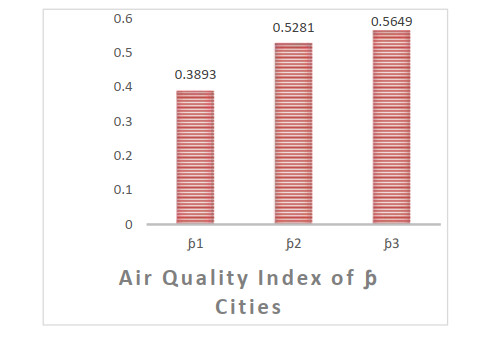
Decision-making in a vague, undetermined and imprecise environment has been a great issue in real-life problems. Many mathematical theories like fuzzy, intuitionistic and neutrosophic sets have been proposed to handle such kinds of environments. Intuitionistic fuzzy sets (IFSS) were formulated by Atanassov in 1986 and analyze the truth membership, which assists in evidence, along with the fictitious membership. This article describes a composition of the intuitionistic fuzzy set (IFS) with the hypersoft set, which assists in coping with multi-attributive decision-making issues. Similarity measures are the tools to determine the similarity index, which evaluates how similar two objects are. In this study, we develop some distance and similarity measures for IFHSS with the help of aggregate operators. Also, we prove some new results, theorems and axioms to check the validity of the proposed study and discuss a real-life problem. The air quality index (AQI) is one of the major factors of the environment which is affected by air pollution. Air pollution is one of the extensive worldwide problems, and now it is well acknowledged to be deleterious to human health. A decision-maker determines ϸ = region (different geographical areas) and the factors$ \{\mathrm{ᵹ}=human~~activiteis,\mathrm{Ϥ}=humidity~~level,\zeta =air~~pollution\} $ which enhance the AQI by applying decision-making techniques. This analysis can be used to determine whether a geographical area has a good, moderate or hazardous AQI. The suggested technique may also be applied to a large number of the existing hypersoft sets. For a remarkable environment, alleviating techniques must be undertaken.

| [1] |
L. A. Zadeh, Fuzzy sets as a basis for a theory of possibility, Fuzzy Set. Syst., 1 (1978), 3–28. https://doi.org/10.1016/0165-0114(78)90029-5 doi: 10.1016/0165-0114(78)90029-5

|
| [2] |
K. M. Lee, K. LEE, K. J. CIOS, Comparison of interval-valued fuzzy sets, intuitionistic fuzzy sets, and bipolar-valued fuzzy sets, Comput. Inform. Technol., 2001,433–439. https://doi.org/10.1142/9789812810885_0055 doi: 10.1142/9789812810885_0055
|
| [3] | C. P. Pappis, C. I. Siettos, T. K. Dasaklis, Fuzzy Sets, systems, and applications, Springer, Boston, MA, 2013. https://doi.org/10.1007/978-1-4419-1153-7_370 |
| [4] |
K. Atanassov, Intuitionistic fuzzy sets, Fuzzy Set. Syst., 20 (1986), 87–96. https://doi.org/10.1016/S0165-0114(86)80034-3 doi: 10.1016/S0165-0114(86)80034-3
|
| [5] | Y. Liu, G. Wang, L. Feng, A general model for transforming vague sets into fuzzy sets, Springer, Berlin, Heidelberg, 2008. https://doi.org/10.1007/978-3-540-87563-5_8 |
| [6] | F. Smarandache, Neutrosophic set a generalization of the intuitionistic fuzzy set, Int. J. Pure Appl. Math., 24 (2005), 287–297. |
| [7] |
D. Molodtsov, Soft set theory first results, Comput. Math. Appl., 37 (1999), 19–31. https://doi.org/10.1016/S0898-1221(99)00056-5 doi: 10.1016/S0898-1221(99)00056-5
|
| [8] |
H. Aktaş, N. Çağman, Soft sets and soft groups, Inform. Sci., 177 (2007), 2726–2735. https://doi.org/10.1016/j.ins.2006.12.008 doi: 10.1016/j.ins.2006.12.008
|
| [9] |
M. I. Ali, F. Feng, X. Liu, W. K. Min, M. Shabir, On some new operations in soft set theory, Comput. Math. Appl., 57 (2009), 1547–1553. https://doi.org/10.1016/j.camwa.2008.11.009 doi: 10.1016/j.camwa.2008.11.009
|
| [10] |
Y. Zou, Z. Xiao, Data analysis approaches of soft sets under incomplete information, Knowl.-Based Syst., 21 (2008), 941–945. https://doi.org/10.1016/j.knosys.2008.04.004 doi: 10.1016/j.knosys.2008.04.004
|
| [11] | P. K. Maji, R. Biswas, A. R. Roy, Fuzzy soft sets, J. Fuzzy Math., 9 (2001), 589–602. |
| [12] |
P. Majumdar, S. K. Samanta, Generalised fuzzy soft sets, Comput. Math. Appl., 59 (2010), 1425–1432. https://doi.org/10.1016/j.camwa.2009.12.006 doi: 10.1016/j.camwa.2009.12.006
|
| [13] | C. Naim, S. Karataş, Intuitionistic fuzzy soft set theory and its decision making, J. Intell. Fuzzy Syst., 24 (2013), 829–836. |
| [14] |
Z. Liang, P. Shi, Similarity measures on intuitionistic fuzzy sets, Pattern Recogn. Lett., 24 (2003), 2687–2693. https://doi.org/10.1016/S0167-8655(03)00111-9 doi: 10.1016/S0167-8655(03)00111-9
|
| [15] |
S. K. De, R. Biswas, A. R. Roy, An application of intuitionistic fuzzy sets in medical diagnosis, Fuzzy Set. Syst., 117 (2001), 209–213. https://doi.org/10.1016/S0165-0114(98)00235-8 doi: 10.1016/S0165-0114(98)00235-8
|
| [16] | P. A. Ejegwa, A. J. Akubo, O. M. Joshua, Intuitionistic fuzzy set and its application in career determination via normalized Euclidean distance method, Eur. Sci. J., 10 (2014), 529–536. |
| [17] |
D. F. Li, Some measures of dissimilarity in intuitionistic fuzzy structures, J. Comput. Syst. Sci., 68 (2004), 115–122. https://doi.org/10.1016/j.jcss.2003.07.006 doi: 10.1016/j.jcss.2003.07.006
|
| [18] | E. Szmidt, J. Kacprzyk, Intuitionistic fuzzy sets in group decision making, Note. Intuition. Fuzzy Set., 2 (1996), 15–32. Available from: http://ifigenia.org/wiki/issue:nifs/2/1/15-32. |
| [19] |
C. P. Wei, P. Wang, Y. Z. Zhang, Entropy, similarity measure of interval-valued intuitionistic fuzzy sets and their applications, Inform. Sci., 181 (2011), 4273–4286. https://doi.org/10.1016/j.ins.2011.06.001 doi: 10.1016/j.ins.2011.06.001
|
| [20] |
M. N. Jafar, A. Saeed, M. Waheed, A. Shafiq, A comprehensive study of intuitionistic fuzzy soft matrices and its applications in selection of laptop by using score function, Int. J. Comput. Appl., 177 (2020), 8–17. https://doi.org/10.5120/ijca2020919844 doi: 10.5120/ijca2020919844
|
| [21] |
B. H. Mitchell, On the Dengfeng-Chuntian similarity measure and its application to pattern recognition, Pattern Recogn. Lett., 24 (2003), 3101–3104. https://doi.org/10.1016/S0167-8655(03)00169-7 doi: 10.1016/S0167-8655(03)00169-7
|
| [22] |
F. Smarandache, Extension of soft set to hypersoft set, and then to plithogenic hypersoft set, Neutrosophic Sets Syst., 22 (2018), 168–170. https://doi.org/10.5281/zenodo.2159754 doi: 10.5281/zenodo.2159754
|
| [23] |
R. M. Zulqarnain, X. L. Xin, M. Saeed, Extension of TOPSIS method under intuitionistic fuzzy hypersoft environment based on correlation coefficient and aggregation operators to solve decision making problem, AIMS Math., 6 (2021), 2732–2755. https://doi.org/10.3934/math.2021167 doi: 10.3934/math.2021167
|
| [24] | A. Yolcu, T. Y. Öztürk, Fuzzy hypersoft sets and its application to decision-making, Theory and Application of Hypersoft Set, Belgium, Brussels: Pons Publishing House, 2021,138–154. |
| [25] |
S. Debnath, Fuzzy hypersoft sets and its weightage operator for decision making, J. Fuzzy Ext. Appl., 2 (2021), 163–170. https://doi.org/10.22105/jfea.2021.275132.1083 doi: 10.22105/jfea.2021.275132.1083
|
| [26] |
A. Yolcu, F. Smarandache, T. Y. Öztürk, Intuitionistic fuzzy hypersoft sets, Commun. Fac. Sci. Univ., 70 (2021), 443–455. https://doi.org/10.31801/cfsuasmas.788329 doi: 10.31801/cfsuasmas.788329
|
| [27] |
R. M. Zulqarnain, I. Siddique, R. Ali, D. Pamucar, D. Marinkovic, D. Bozanic, Robust aggregation operators for intuitionistic fuzzy hypersoft set with their application to solve mcdm problem, Entropy, 23 (2021), 688. https://doi.org/10.3390/e23060688 doi: 10.3390/e23060688
|
| [28] |
R. M. Zulqarnain, I. Siddique, F. Jarad, H. Karamti, A. Iampan, Aggregation operators for interval-valued intuitionistic fuzzy hypersoft set with their application in material selection, Math. Probl. Eng., 2022, 1–21. https://doi.org/10.1155/2022/8321964 doi: 10.1155/2022/8321964
|
| [29] |
A. Ashraf, K. Ullah, A. Hussain, M. Bari, Interval-valued picture fuzzy Maclaurin symmetric mean operator with application in multiple attribute decision-making, Rep. Mech. Eng., 3 (2022), 301–317. https://doi.org/10.31181/rme20020042022a doi: 10.31181/rme20020042022a
|
| [30] |
M. Riaz, H. M. A. Farid, Picture fuzzy aggregation approach with application to third-party logistic provider selection process, Rep. Mech. Eng., 3 (2022), 318–327. https://doi.org/10.31181/rme20023062022r doi: 10.31181/rme20023062022r
|
| [31] |
S. Broumi, R. Sundareswaran, M. Shanmugapriya, G. Nordo, M. Talea, A. Bakali, et al., Interval- valued fermatean neutrosophic graphs, Decis. Making Appl. Manag. Eng., 5 (2022), 176–200. https://doi.org/10.31181/dmame0311072022b doi: 10.31181/dmame0311072022b
|
| [32] |
A. K. Das, C. Granados, FP-intuitionistic multi fuzzy N-soft set and its induced FP-Hesitant N soft set in decision-making, Decis. Making Appl. Manag. Eng., 5 (2022), 67–89. https://doi.org/10.31181/dmame181221045d doi: 10.31181/dmame181221045d
|
| [33] |
S. Das, R. Das, S. Pramanik, Single valued pentapartitioned neutrosophic graphs, Neutrosophic Sets Syst., 50 (2022), 225–238. https://doi.org/10.5281/zenodo.6774779 doi: 10.5281/zenodo.6774779
|
| [34] |
M. H. Sowlat, H. Gharibi, M. Yunesian, M. T. Mahmoudi, S. Lotfi, A novel, fuzzy-based air quality index (FAQI) for air quality assessment, Atmos. Environ., 45 (2011), 2050–2059. https://doi.org/10.1016/j.atmosenv.2011.01.060 doi: 10.1016/j.atmosenv.2011.01.060
|
| [35] |
A. Kumar, P. Goyal, Forecasting of daily air quality index in Delhi, Sci. Total Environ., 409 (2011), 5517–5523. https://doi.org/10.1016/j.scitotenv.2011.08.069 doi: 10.1016/j.scitotenv.2011.08.069
|
| [36] |
D. Zhan, M. P. Kwan, W. Zhang, X. Yu, B. Meng, Q. Liu, The driving factors of air quality index in China, J. Clean. Prod., 197 (2018), 1342–1351. https://doi.org/10.1016/j.jclepro.2018.06.108 doi: 10.1016/j.jclepro.2018.06.108
|
| [37] |
M. Saqlain, S. Moin, M. N. Jafar, M. Saeed, S. Broumi, Single and multi-valued neutrosophic hypersoft set and tangent similarity measure of single valued neutrosophic hypersoft sets, Neutrosophic Sets Syst., 32 (2020), 317–329. https://doi.org/10.5281/zenodo.3723165 doi: 10.5281/zenodo.3723165
|
| [38] |
M. N. Jafar, M. Saeed, M. Saqlain, M. S. Yang, Trigonometric similarity measures for neutrosophic hypersoft sets with application to renewable energy source selection, IEEE Access, 9 (2021), 129178–129187. https://doi.org/10.1109/ACCESS.2021.3112721 doi: 10.1109/ACCESS.2021.3112721
|
| [39] |
M. Riaz, M. R. Hashmi, Linear Diophantine fuzzy set and its applications towards multi-attribute decision-making problems, J. Intell. Fuzzy Syst., 37 (2019), 5417–5439. https://doi.org/10.3233/JIFS-190550 doi: 10.3233/JIFS-190550
|
| [40] |
M. Riaz, R. M. Hashmi, D. Pamucar, Y. M. Chu, Spherical linear Diophantine fuzzy sets with modeling uncertainties in MCDM, Comp. Model. Eng. Sci., 126 (2021), 1125–1164. https://doi.org/10.32604/cmes.2021.013699 doi: 10.32604/cmes.2021.013699
|
| [41] |
M. Riaz, A. Habib, M. Saqlain, M. S. Yang, Cubic bipolar fuzzy-VIKOR method using new distance and entropy measures and Einstein averaging aggregation operators with application to renewable energy, Int. J. Fuzzy Syst., 2022, 1–34. https://doi.org/10.1007/s40815-022-01383-z doi: 10.1007/s40815-022-01383-z
|
| [42] |
S. Y. Musa, B. A. Asaad, Bipolar hypersoft sets, Mathematics, 9 (2021), 1826. https://doi.org/10.3390/math9151826 doi: 10.3390/math9151826
|
| [43] |
F. Smarandache, Introduction to the indetermsoft set and indetermhypersoft set, Neutrosophic Sets Sy., 50 (2022), 629–650. https://doi.org/10.5281/zenodo.6774960 doi: 10.5281/zenodo.6774960
|
Figures(1) / Tables(19)

Muhammad Saqlain, Muhammad Riaz, Raiha Imran, Fahd Jarad. Distance and similarity measures of intuitionistic fuzzy hypersoft sets with application: Evaluation of air pollution in cities based on air quality index[J]. AIMS Mathematics, 2023, 8(3): 6880-6899. doi: 10.3934/math.2023348


 DownLoad: