Study of nonlinear thermal convection of ternary nanofluid within Darcy-Brinkman porous structure with time dependent heat source/sink

Kiran Sajjan; N. Ameer Ahammad; C. S. K. Raju; M. Karuna Prasad; Nehad Ali Shah; Thongchai Botmart; Kiran Sajjan; N. Ameer Ahammad; C. S. K. Raju; M. Karuna Prasad; Nehad Ali Shah; Thongchai Botmart

doi:10.3934/math.2023211

AIMS Mathematics

2023, Volume 8, Issue 2: 4237-4260. doi: 10.3934/math.2023211

Previous Article Next Article

Research article

Study of nonlinear thermal convection of ternary nanofluid within Darcy-Brinkman porous structure with time dependent heat source/sink

1.
Department of Mathematics, GITAM School of Science, GITAM Deemed to be University, Bangalore-Campus, Karnataka 562163, India
2.
Department of Mathematics, Faculty of Science, University of Tabuk, P.O. Box741, Tabuk 71491, Saudi Arabia
3.
Department of Mechanical Engineering, Sejong University, Seoul 05006, South Korea
4.
Department of Mathematics, Faculty of Science, Khon Kaen University, Khon Kaen 40002, Thailand
^† These authors contributed equally to this work and are co-first authors

Received: 25 July 2022 Revised: 13 October 2022 Accepted: 18 October 2022 Published: 02 December 2022
MSC : 76–10, 76R10

The dynamical behaviour and thermal transportation feature of mixed convective Casson bi-phasic flows of water-based ternary Hybrid nanofluids with different shapes are examined numerically in a Darcy- Brinkman medium bounded by a vertical elongating slender concave-shaped surface. The mathematical framework of the present flow model is developed properly by adopting the single-phase approach, whose solid phase is selected to be metallic or metallic oxide nanoparticles. Besides, the influence of thermal radiation is taken into consideration in the presence of an internal variable heat generation. A set of feasible similarity transformations are applied for the conversion of the governing PDEs into a nonlinear differential structure of coupled ODEs. An advanced differential quadrature algorithm is employed herein to acquire accurate numerical solutions for momentum and energy equations. Results of the conducted parametric study are explained and revealed in graphs using bvp5c in MATLAB to solve the governing system. The solution with three mixture compositions is provided (Type-I and Type-II). Al₂O₃ (Platelet), GNT (Cylindrical), and CNTs (Spherical), Type-II mixture of copper (Cylindrical), silver (Platelet), and copper oxide (Spherical). In comparison to Type-I ternary combination Type-II ternary mixtures is lesser in terms of the temperature distribution. The skin friction coefficient is more in Type-1 compared to Type-2.
- thermal radiation,
- Casson rheological model,
- ternary hybrid nanofluid,
- porous medium,
- irregular geometry,
- local skin friction coefficients
Citation: Kiran Sajjan, N. Ameer Ahammad, C. S. K. Raju, M. Karuna Prasad, Nehad Ali Shah, Thongchai Botmart. Study of nonlinear thermal convection of ternary nanofluid within Darcy-Brinkman porous structure with time dependent heat source/sink[J]. AIMS Mathematics, 2023, 8(2): 4237-4260. doi: 10.3934/math.2023211

Related Papers:

Abstract

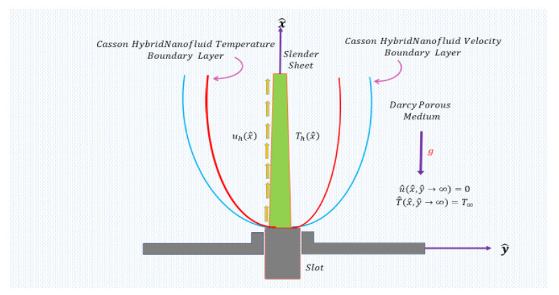
The dynamical behaviour and thermal transportation feature of mixed convective Casson bi-phasic flows of water-based ternary Hybrid nanofluids with different shapes are examined numerically in a Darcy- Brinkman medium bounded by a vertical elongating slender concave-shaped surface. The mathematical framework of the present flow model is developed properly by adopting the single-phase approach, whose solid phase is selected to be metallic or metallic oxide nanoparticles. Besides, the influence of thermal radiation is taken into consideration in the presence of an internal variable heat generation. A set of feasible similarity transformations are applied for the conversion of the governing PDEs into a nonlinear differential structure of coupled ODEs. An advanced differential quadrature algorithm is employed herein to acquire accurate numerical solutions for momentum and energy equations. Results of the conducted parametric study are explained and revealed in graphs using bvp5c in MATLAB to solve the governing system. The solution with three mixture compositions is provided (Type-I and Type-II). Al₂O₃ (Platelet), GNT (Cylindrical), and CNTs (Spherical), Type-II mixture of copper (Cylindrical), silver (Platelet), and copper oxide (Spherical). In comparison to Type-I ternary combination Type-II ternary mixtures is lesser in terms of the temperature distribution. The skin friction coefficient is more in Type-1 compared to Type-2.

References

[1]	H. Yarmand, S. Gharehkhani, G. Ahmadi, S. F. S. Shirazi, S. Baradaran, E. Montazer, et al., Graphene nanoplatelets-silver hybrid nanofluids for enhanced heat transfer, Energy Convers. Management, 100 (2015), 419–428. https://doi.org/10.1016/j.enconman.2015.05.023 doi: 10.1016/j.enconman.2015.05.023
[2]	O. K. Koriko, K. S. Adegbie, I. L. Animasaun, M. A. Olotu, Numerical solutions of the partial differential equations for investigating the significance of partial slip due to lateral velocity and viscous dissipation: the case of blood-gold Carreau nanofluid and dusty fluid, Numer. Methods Part. Differ. Equ., 2021. https://doi.org/10.1002/num.22754 doi: 10.1002/num.22754
[3]	Y. N. Jiang, X. M. Zhou, Y. Wang, Effects of nanoparticle shapes on heat and mass transfer of nanofluid thermocapillary convection around a gas bubble, Microgravity Sci. Technol., 32 (2020), 167–177.
[4]	M. C. Arno, M. Inam, A. C. Weems, Z. Li, A. L. A. Binch, C. I. Platt, et al., Exploiting the role of nanoparticle shape in enhancing hydrogel adhesive and mechanical properties, Nat. commun., 11 (2020), 1–9.
[5]	L. Th. Benos, E. G. Karvelas, I. E. Sarris, A theoretical model for the manetohydrodynamic natural convection of a CNT-water nanofluid incorporating a renovated Hamilton-Crosser model, Int. J. Heat Mass Trans., 135 (2019), 548–560. https://doi.org/10.1016/j.ijheatmasstransfer.2019.01.148 doi: 10.1016/j.ijheatmasstransfer.2019.01.148
[6]	H. Liu, I. L. Animasaun, N. A. Shah, O. K. Koriko, B. Mahanthesh, Further discussion on the significance of quartic autocatalysis on the dynamics of water conveying 47 nm alumina and 29 nm cupric nanoparticles, Arab. J. Sci. Eng., 45 (2020), 5977–6004.
[7]	A. S. Sabu, A. Wakif, S. Areekara, A. Mathew, N. A. Shah, Significance of nanoparticles' shape and thermo-hydrodynamic slip constraints on MHD alumina-water nanoliquid flows over a rotating heated disk: the passive control approach, Int. Commun. Heat Mass Trans., 129 (2021), 105711. https://doi.org/10.1016/j.icheatmasstransfer.2021.105711 doi: 10.1016/j.icheatmasstransfer.2021.105711
[8]	Q. Lou, B. Ali, S. U. Rehman, D. Habib, S. Abdal, N. A. Shah, et al., Micropolar dusty fluid: Coriolis force effects on dynamics of MHD rotating fluid when Lorentz force is significant, Mathematics, 10 (2022), 2630. https://doi.org/10.3390/math10152630 doi: 10.3390/math10152630
[9]	M. Z. Ashraf, S. U. Rehman, S. Farid, A. K. Hussein, B. Ali, N. A. Shah, et al., Insight into significance of bioconvection on MHD tangent hyperbolic nanofluid flow of irregular thickness across a slender elastic surface, Mathematics, 10 (2022), 2592. https://doi.org/10.3390/math10152592 doi: 10.3390/math10152592
[10]	K. Vajravelu, Convection heat transfer at a stretching sheet with suction or blowing, J. Math. Anal. Appl., 188 (1994), 1002–1011. https://doi.org/10.1006/jmaa.1994.1476 doi: 10.1006/jmaa.1994.1476
[11]	C-K. Chen, M-I. Char, Heat transfer of a continuous, stretching surface with suction or blowing, J. Math. Anal. Appl., 135 (1988), 568–580. https://doi.org/10.1016/0022-247X(88)90172-2 doi: 10.1016/0022-247X(88)90172-2
[12]	R. N. Kumar, R. J. P. Gowda, A. M. Abusorrah, Y. M. Mahrous, N. H. Abu-Hamdeh, A. Issakhov, et al., Impact of magnetic dipole on ferromagnetic hybrid nanofluid flow over a stretching cylinder, Phys. Scr., 96 (2021), 045215. https://doi.org/10.1088/1402-4896/abe324 doi: 10.1088/1402-4896/abe324
[13]	B. Ali, I. Siddique, I. Khan, B. Masood, S. Hussain, Magnetic dipole and thermal radiation effects on hybrid base micropolar CNTs flow over a stretching sheet: finite element method approach, Results Phys., 25 (2021), 104145. https://doi.org/10.1016/j.rinp.2021.104145 doi: 10.1016/j.rinp.2021.104145
[14]	G. C. Rana, S. K. Kango, Effect of rotation on thermal instability of compressible Walters' (Model B′) fluid in porous medium, J. Adv. Res. Appl. Math., 3 (2011), 44–57. https://doi.org/10.5373/jaram.815.030211 doi: 10.5373/jaram.815.030211
[15]	A. V. Kuznetsov, D. A. Nield, Thermal instability in a porous medium layer saturated by a nanofluid: Brinkman model, Transp. Porous Media, 81 (2010), 409–422.
[16]	L. J. Sheu, Linear stability of convection in a viscoelastic nanofluid layer, Eng. Int. J. Mech. Mechatron. Eng., 5 (2011), 1970–1976.
[17]	L. L. Lee, Boundary layer over a thin needle, Phys. Fluids, 10 (1967), 820–822. https://doi.org/10.1063/1.1762194 doi: 10.1063/1.1762194
[18]	J. L. S. Chen, Mixed convection flow about slender bodies of revolution, ASME J. Heat Mass Trans., 109 (1987), 1033–1036. https://doi.org/10.1115/1.3248177 doi: 10.1115/1.3248177
[19]	T. Fang, J. Zhang, Y. Zhong, Boundary layer flow over a stretching sheet with variable thickness, Appl. Math. Comput., 218 (2012), 7241–7252. https://doi.org/10.1016/j.amc.2011.12.094 doi: 10.1016/j.amc.2011.12.094
[20]	R. Jusoh, R. Nazar, I. Pop, Three-dimensional flow of a nanofluid over a permeable stretching/shrinking surface with velocity slip: A revised model, Phys. Fluids, 30 (2018), 033604. https://doi.org/10.1063/1.5021524 doi: 10.1063/1.5021524
[21]	A. Jamaludin, R. Nazar, I. Pop, Three-dimensional magnetohydrodynamic mixed convection flow of nanofluids over a nonlinearly permeable stretching/shrinking sheet with velocity and thermal slip, Appl. Sci., 8 (2018), 1128. https://doi.org/10.3390/app8071128 doi: 10.3390/app8071128
[22]	N. S. Khashi'ie, N. M. Arifin, R. Nazar, E. H. Hafidzuddin, N. Wahi, I. Pop, A stability analysis for magnetohydrodynamics stagnation point flow with zero nanoparticles flux condition and anisotropic slip, Energies, 12 (2019), 1268. https://doi.org/10.3390/en12071268 doi: 10.3390/en12071268
[23]	P. Rana, A. Kumar, G. Gupta, Impact of different arrangements of heated elliptical body, fins and differential heater in MHD convective transport phenomena of inclined cavity utilizing hybrid nanoliquid: Artificial neutral network prediction, Int. Commun. Heat Mass Trans., 132 (2022), 105900. https://doi.org/10.1016/j.icheatmasstransfer.2022.105900 doi: 10.1016/j.icheatmasstransfer.2022.105900
[24]	C. S. K. Raju, N. A. Ahammad, K. Sajjan, N. A. Shah, S-J. Yook, M. D. Kumar, Nonlinear movements of axisymmetric ternary hybrid nanofluids in a thermally radiated expanding or contracting permeable Darcy Walls with different shapes and densities: simple linear regression, Int. Commun. Heat Mass Trans., 135 (2022), 106110. https://doi.org/10.1016/j.icheatmasstransfer.2022.106110 doi: 10.1016/j.icheatmasstransfer.2022.106110
[25]	P. Rana, S. Gupta, G. Gupta, Unsteady nonlinear thermal convection flow of MWCNT-MgO/EG hybrid nanofluid in the stagnation-point region of a rotating sphere with quadratic thermal radiation: RSM for optimization, Int. Commun. Heat Mass Trans., 134 (2022), 106025. https://doi.org/10.1016/j.icheatmasstransfer.2022.106025 doi: 10.1016/j.icheatmasstransfer.2022.106025
[26]	N. A. Shah, A. Wakif, E. R. El-Zahar, T. Thumma, S.-J. Yook, Heat transfers thermodynamic activity of a second-grade ternary nanofluid flow over a vertical plate with Atangana-Baleanu time-fractional integral, Alexandria Eng. J., 61 (2022), 10045–10053. https://doi.org/10.1016/j.aej.2022.03.048 doi: 10.1016/j.aej.2022.03.048
[27]	R. Zhang, N. A. Ahammad, C. S. K. Raju, S. M. Upadhya, N. A. Shah, S-J. Yook, Quadratic and linear radiation impact on 3D convective hybrid nanofluid flow in a suspension of different temperature of waters: transpiration and fourier fluxes, Int. Commun. Heat Mass Trans., 138 (2022), 106418. https://doi.org/10.1016/j.icheatmasstransfer.2022.106418 doi: 10.1016/j.icheatmasstransfer.2022.106418
[28]	N. Acharya, Spectral quasi linearization simulation on the radiative nanofluid spraying over a permeable inclined spinning disk considering the existence of heat source/sink, Appl. Math. Comput., 411 (2021), 126547. https://doi.org/10.1016/j.amc.2021.126547 doi: 10.1016/j.amc.2021.126547
[29]	P. Rana, W. Al-Kouz, B. Mahanthesh, J. Mackolil, Heat transfer of TiO2-EG nanoliquid with active and passive control of nanoparticles subject to nonlinear Boussinesq approximation, Int. Commun. Heat Mass Trans., 126 (2021), 105443. https://doi.org/10.1016/j.icheatmasstransfer.2021.105443 doi: 10.1016/j.icheatmasstransfer.2021.105443
[30]	T. Elnaqeeb, I. L. Animasaun, N. A. Shah, Ternary-hybrid nanofluids: significance of suction and dual-stretching on three-dimensional flow of water conveying nanoparticles with various shapes and densities, Z. Naturforsch. A, 76 (2021). https://doi.org/10.1515/zna-2020-0317 doi: 10.1515/zna-2020-0317
[31]	N. A. Shah, A. Wakif, E. R. El-Zahar, S. Ahmad, S-J Yook, Numerical simulation of a thermally enhanced EMHD flow of a heterogeneous micropolar mixture comprising (60%)-ethylene glycol (EG), (40%)-water (W), and copper oxide nanomaterials (CuO), Case Study. Therm. Eng., 35 (2022), 102046. https://doi.org/10.1016/j.csite.2022.102046 doi: 10.1016/j.csite.2022.102046
[32]	M. S. Upadhya, C. S. K. Raju, Implementation of boundary value problems in using MATLAB®, In: Micro and nanofluid convection with magnetic field effects for heat and mass transfer applications using MATLAB, Elsevier, 2022,169–238. https://doi.org/10.1016/B978-0-12-823140-1.00010-5
[33]	M. Khader, A. M. Megahed, Numerical solution for boundary layer flow due to a nonlinearly stretching sheet with variable thickness and slip velocity, Eur. Phys. J. Plus, 128 (2013), 100–108.

Reader Comments

Your name:*

Email:*
© 2023 the Author(s), licensee AIMS Press. This is an open access article distributed under the terms of the Creative Commons Attribution License (http://creativecommons.org/licenses/by/4.0)