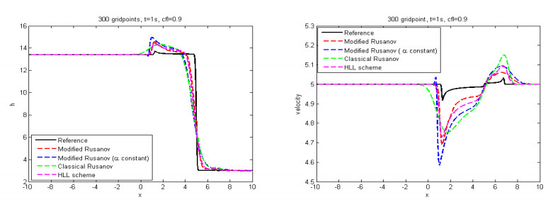
In this work, we consider the model of shallow water equation with horizontal density gradients. We develop the modified Rusanov (mR) scheme to solve this model in one and two dimensions. Predictor and corrector are the two stages of the suggested scheme. The predictor stage is dependent on a local parameter $ (\alpha^n_{i+\frac{1}{2}}) $ that allows for diffusion control. The balance conservation equation is recovered in the corrector stage. The proposed approach is well-balanced, conservative, and straightforward. Several 1D and 2D test cases are produced after presenting the shallow water model and the numerical technique. In the 1D case, we compared the proposed scheme with the Rusanov scheme, mR with constant $ \alpha $ and analytical solutions. The numerical simulation demonstrates the mR's great resolution and attests to its capacity to produce accurate simulations of the shallow water equation with horizontal density gradients. Our results demonstrate that the mR technique is a highly effective instrument for solving a variety of equations in applied science and developed physics.
Citation: Kamel Mohamed, H. S. Alayachi, Mahmoud A. E. Abdelrahman. The mR scheme to the shallow water equation with horizontal density gradients in one and two dimensions[J]. AIMS Mathematics, 2023, 8(11): 25754-25771. doi: 10.3934/math.20231314
In this work, we consider the model of shallow water equation with horizontal density gradients. We develop the modified Rusanov (mR) scheme to solve this model in one and two dimensions. Predictor and corrector are the two stages of the suggested scheme. The predictor stage is dependent on a local parameter $ (\alpha^n_{i+\frac{1}{2}}) $ that allows for diffusion control. The balance conservation equation is recovered in the corrector stage. The proposed approach is well-balanced, conservative, and straightforward. Several 1D and 2D test cases are produced after presenting the shallow water model and the numerical technique. In the 1D case, we compared the proposed scheme with the Rusanov scheme, mR with constant $ \alpha $ and analytical solutions. The numerical simulation demonstrates the mR's great resolution and attests to its capacity to produce accurate simulations of the shallow water equation with horizontal density gradients. Our results demonstrate that the mR technique is a highly effective instrument for solving a variety of equations in applied science and developed physics.

| [1] |
G. Hernandez-Duenas, A hybrid method to solve shallow water flows with horizontal density gradients, J. Sci. Comput., 73 (2017), 753–782. https://doi.org/10.1007/s10915-017-0553-1 doi: 10.1007/s10915-017-0553-1

|
| [2] |
V. A. Dorodnitsyn, E. I. Kaptsov, Discrete shallow water equations preserving symmetries and conservation laws, J. Math. Phys., 62 (2021), 083508. https://doi.org/10.1063/5.0031936 doi: 10.1063/5.0031936
|
| [3] |
V. A. Dorodnitsyn, E. I. Kaptsov, Shallow water equations in Lagrangian coordinates: symmetries, conservation laws and its preservation in difference models, Commun. Nonlinear Sci. Numer. Simul., 89 (2020), 105343. https://doi.org/10.1016/j.cnsns.2020.105343 doi: 10.1016/j.cnsns.2020.105343
|
| [4] | E. Godlewski, P. A. Raviart, Numerical approximation of hyperbolic systems of conservation laws, Springer, New York, 1996. https://doi.org/10.1007/978-1-4612-0713-9 |
| [5] | L. C. Evans, Partial differential equations, American Mathematical Society, 1998. |
| [6] | R. J. LeVeque, Finite volume methods for hyperbolic problems, Cambridge University Press, 2002. https://doi.org/10.1017/CBO9780511791253 |
| [7] |
M. A. E. Abdelrahman, On the shallow water equations, Z. Naturforschung A, 72 (2017), 873–879. https://doi.org/10.1515/zna-2017-0146 doi: 10.1515/zna-2017-0146
|
| [8] |
K. Mohamed, M. A. E. Abdelrahman, The modified Rusanov scheme for solving the ultra-relativistic Euler equations, Eur. J. Mech.-B/Fluids, 90 (2021), 89–98. https://doi.org/10.1016/j.euromechflu.2021.07.014 doi: 10.1016/j.euromechflu.2021.07.014
|
| [9] |
M. A. E. Abdelrahman, On the shallow water equations, Z. Naturforschung A, 72 (2017), 873–879. https://doi.org/10.1515/zna-2017-0146 doi: 10.1515/zna-2017-0146
|
| [10] | E. F. Toro, Riemann solvers and numerical methods for fluid dynamics, Springer Berlin, Heidelberg, 1999. https://doi.org/10.1007/b79761 |
| [11] |
Z. Fu, Z. Tang, Q. Xi, Q. Liu, Y. Gu, F. Wang, Localized collocation schemes and their applications, Acta Mech. Sin., 38 (2022), 422167. https://doi.org/10.1007/s10409-022-22167-x doi: 10.1007/s10409-022-22167-x
|
| [12] |
Z. J. Fu, Z. Y. Xie, S. Y. Ji, C. C. Tsai, A. L. Li, Meshless generalized finite difference method for water wave interactions with multiple-bottom-seated-cylinder-array structures, Ocean Eng., 195 (2020), 106736. https://doi.org/10.1016/j.oceaneng.2019.106736 doi: 10.1016/j.oceaneng.2019.106736
|
| [13] |
A. R. Alharbi, M. B. Almatrafi, New exact and numerical solutions with their stability for Ito integro-differential equation via Riccati–Bernoulli sub-ODE method, J. Taibah Univ. Sci., 14 (2020), 1447–1456. https://doi.org/10.1080/16583655.2020.1827853 doi: 10.1080/16583655.2020.1827853
|
| [14] |
M. A. E. Abdelrahman, M. B. Almatrafi, A. Alharbi, Fundamental solutions for the coupled KdV system and its stability, Symmetry, 12 (2020), 429. https://doi.org/10.3390/sym12030429 doi: 10.3390/sym12030429
|
| [15] |
M. A. E. Abdelrahman, A. Alharbi, Analytical and numerical investigations of the modified Camassa-Holm equation, Pramana-J. Phys., 95 (2021), 117. https://doi.org/10.1007/s12043-021-02153-6 doi: 10.1007/s12043-021-02153-6
|
| [16] | K. Mohamed, Simulation numérique en volume finis, de problémes d'écoulements multidimensionnels raides, par un schéma de flux á deux pas, Doctoral dissertation, Université Paris-Nord-Paris XIII, 2005. |
| [17] |
K. Mohamed, M. Seaid, M. Zahri, A finite volume method for scalar conservation laws with stochastic time-space dependent flux function, J. Comput. Appl. Math., 237 (2013), 614–632. https://doi.org/10.1016/j.cam.2012.07.014 doi: 10.1016/j.cam.2012.07.014
|
| [18] | F. Benkhaldoun, K. Mohamed, M. Seaid, A generalized Rusanov method for Saint-Venant equations with variable horizontal density, In: J. Foõt, J. Fürst, J. Halama, R. Herbin, F. Hubert, Finite volumes for complex applications VI problems & perspectives, Springer Proceedings in Mathematics, Springer, Berlin, Heidelberg, 4 (2011), 89–96. https://doi.org/10.1007/978-3-642-20671-9_10 |
| [19] |
K. Mohamed, F. Benkhaldoun, A modified Rusanov scheme for shallow water equations with topography and two phase flows, Eur. Phys. J. Plus, 131 (2016), 207. https://doi.org/10.1140/epjp/i2016-16207-3 doi: 10.1140/epjp/i2016-16207-3
|
| [20] |
K. Mohamed, H. A. Alkhidhr, M. A. E. Abdelrahman, The NHRS scheme for the Chaplygin gas model in one and two dimensions, AIMS Math., 7 (2022), 17785–17801. https://doi.org/10.3934/math.2022979 doi: 10.3934/math.2022979
|
| [21] |
K. Mohamed, M. A. E. Abdelrahman, The NHRS scheme for the two models of traffic flow, Comp. Appl. Math., 42 (2023), 53. https://doi.org/10.1007/s40314-022-02172-y doi: 10.1007/s40314-022-02172-y
|
| [22] |
K. Mohamed, S. Sahmim, M. A. E. Abdelrahman, A Predictor-corrector scheme for simulation of two-phase granular flows over a moved bed with a variable topography, Eur. J. Mech.-B/Fluids, 96 (2022), 39–50. https://doi.org/10.1016/j.euromechflu.2022.07.001 doi: 10.1016/j.euromechflu.2022.07.001
|
| [23] |
M. Dumbser, D. S. Balsara, A new efficient formulation of the HLLM Riemann solver for general conservative and non-conservative hyperbolic systems, J. Comput. Phys., 304 (2016), 275–319. https://doi.org/10.1016/j.jcp.2015.10.014 doi: 10.1016/j.jcp.2015.10.014
|
| [24] |
R. J. LeVeque, Balancing source terms and flux gradients in high-resolution godynov methods: the quasi-steady wave propagation algorithm, J. Comput. Phys., 146 (1998), 346–365. https://doi.org/10.1006/jcph.1998.6058 doi: 10.1006/jcph.1998.6058
|
| [25] |
L. Gosse, A well-balanced scheme using non-conservative products designed for hyperbolic systems of conservation laws with source terms, Math. Models Methods Appl. Sci., 11 (2001), 339–365. https://doi.org/10.1142/S021820250100088X doi: 10.1142/S021820250100088X
|
| [26] |
A. Bermudez, M. E. Vazquez, Upwind methods for hyperbolic conservation laws with source term, Comput. Fluids, 23 (1994), 1049–1071. https://doi.org/10.1016/0045-7930(94)90004-3 doi: 10.1016/0045-7930(94)90004-3
|


Figures(20)

Kamel Mohamed, H. S. Alayachi, Mahmoud A. E. Abdelrahman. The mR scheme to the shallow water equation with horizontal density gradients in one and two dimensions[J]. AIMS Mathematics, 2023, 8(11): 25754-25771. doi: 10.3934/math.20231314


 DownLoad: