On the reach and the smoothness class of pipes and offsets: a survey

Javier Sánchez-Reyes; Leonardo Fernández-Jambrina; Javier Sánchez-Reyes; Leonardo Fernández-Jambrina

doi:10.3934/math.2022435

AIMS Mathematics

2022, Volume 7, Issue 5: 7742-7758. doi: 10.3934/math.2022435

Previous Article Next Article

Survey

On the reach and the smoothness class of pipes and offsets: a survey

Javier Sánchez-Reyes ^{1
,
,},
Leonardo Fernández-Jambrina ²

1.
IMACI, ETS Ingeniería Industrial, Campus Universitario, Edificio Politécnico, Universidad de Castilla-La Mancha, 13071-Ciudad Real, Spain
2.
Dep. de Matemática e Informática Aplicadas a las Ingenierías Civil y Naval, Universidad Politécnica de Madrid, Av. de la Memoria 4, 28040-Madrid, Spain

Received: 13 December 2021 Revised: 07 February 2022 Accepted: 10 February 2022 Published: 17 February 2022
MSC : 53-A04, 53-A05, 65-D17

Pipes and offsets are the sets obtained by displacing the points of their progenitor $ S $ (i.e., spine curve or base surface, respectively) a constant distance $ d $ along normal lines. We review existing results and elucidate the relationship between the smoothness of pipes/offsets and the reach $ R $ of the progenitor, a fundamental concept in Federer's celebrated paper where he introduced the family of sets with positive reach. Most CAD literature on pipes/offsets overlooks this concept despite its relevance, so we remedy this deficiency with this survey. The reach admits a geometric interpretation, as the minimal distance between $ S $ and its cut locus. For a closed $ S $, the condition $ d < R $ means a singularity-free pipe/offset, coinciding with the level set at a distance $ d $ from the progenitor. This condition also implies that pipes/offsets inherit the smoothness class $ C^k $, $ k\ge1 $, of a closed progenitor. These results hold in spaces of arbitrary dimension, for pipe hypersurfaces from spines or offsets to base hypersurfaces.
- cut locus,
- level set,
- offset,
- pipe,
- progenitor,
- reach,
- smoothness class,
- spine
Citation: Javier Sánchez-Reyes, Leonardo Fernández-Jambrina. On the reach and the smoothness class of pipes and offsets: a survey[J]. AIMS Mathematics, 2022, 7(5): 7742-7758. doi: 10.3934/math.2022435

Related Papers:

Abstract

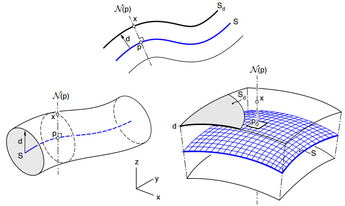
Pipes and offsets are the sets obtained by displacing the points of their progenitor $ S $ (i.e., spine curve or base surface, respectively) a constant distance $ d $ along normal lines. We review existing results and elucidate the relationship between the smoothness of pipes/offsets and the reach $ R $ of the progenitor, a fundamental concept in Federer's celebrated paper where he introduced the family of sets with positive reach. Most CAD literature on pipes/offsets overlooks this concept despite its relevance, so we remedy this deficiency with this survey. The reach admits a geometric interpretation, as the minimal distance between $ S $ and its cut locus. For a closed $ S $, the condition $ d < R $ means a singularity-free pipe/offset, coinciding with the level set at a distance $ d $ from the progenitor. This condition also implies that pipes/offsets inherit the smoothness class $ C^k $, $ k\ge1 $, of a closed progenitor. These results hold in spaces of arbitrary dimension, for pipe hypersurfaces from spines or offsets to base hypersurfaces.

References

[1]	R. E. Barnhill, Geometry Processing for Design and Manufacturing, Philadelphia: SIAM, 1992.
[2]	N. M. Patrikalakis, T. Maekawa, Shape interrogation for Computer Aided Design and Manufacturing, Berlin: Springer, 2002.
[3]	J. Hoschek, D. Lasser, Fundamentals of Computer Aided Geometric Design, Wellesley, MA: AK Peters, 1993.
[4]	H. Pottmann, A. Asperl, M. Hofer, A. Kilian, Architectural geometry, Exton: Bentley Institute Press, 2007.
[5]	H. Pottmann, M. Eigensatz, A. Vaxman, J. Wallner, Architectural geometry, Comput. Graph., 47 (2015), 145–164. https://doi.org/10.1016/j.cag.2014.11.002
[6]	T. Maekawa, N. M. Patrikalakis, T. Sakkalis, G. Yu, Analysis and applications of pipe surfaces, Comput. Aided Geom. Des., 15 (1998), 437–458. https://doi.org/10.1016/S0167-8396(97)00042-3 doi: 10.1016/S0167-8396(97)00042-3
[7]	M. do Carmo, Differential Geometry of Curves and Surfaces, Upper Saddle River, NJ: Prentice-Hall, 1976.
[8]	A. Gray, E. Abbena, S. Salomon, Modern Differential Geometry of Curves and Surfaces with Mathematica, 3rd Ed., Boca Raton, FL: Chapman & Hall/CRC, 2006.
[9]	T. Maekawa, An overview of offset curves and surfaces, Comput.-Aided Des., 31 (1999), 165–163. https://doi.org/10.1016/S0010-4485(99)00013-5 doi: 10.1016/S0010-4485(99)00013-5
[10]	J. G. Alcázar, J. R. Sendra, Local shape of offsets to algebraic curves, J. Symb. Comput., 42 (2007), 38–351. https://doi.org/10.1016/j.jsc.2006.12.001 doi: 10.1016/j.jsc.2006.12.001
[11]	J. G. Alcázar, Good local behavior of offsets to rational regular algebraic surfaces, J. Symb. Comput., 43 (2008), 845–857. https://doi.org/10.1016/j.jsc.2008.04.001 doi: 10.1016/j.jsc.2008.04.001
[12]	J. G. Alcázar, Good global behavior of offsets to plane algebraic curves J. Symb. Comput., 43 (2008), 659–680. https://doi.org/10.1016/j.jsc.2008.01.003
[13]	H. Federer, Curvature measures, Trans. Amer. Math. Soc., 93 (1959), 418–491.
[14]	J. Wallner, T. Sakkalis, T. Maekawa, H. Pottmann, G. Yu, Self-intersections of offset curves and surfaces, International Journal of Shape Modeling, 7 (2001), 1–21. https://doi.org/10.1142/S0218654301000023 doi: 10.1142/S0218654301000023
[15]	T. Sakkalis, T. J. Peters, J. Bisceglio, Isotopic approximations and interval solids, Comput.-Aided Des., 36 (2014), 1089–1100. https://doi.org/10.1016/j.cad.2004.01.008 doi: 10.1016/j.cad.2004.01.008
[16]	T. Hermann, On the smoothness of offset surfaces, Comput. Aided Geom. Des., 15 (1998), 529–533. https://doi.org/10.1016/S0167-8396(98)00002-8 doi: 10.1016/S0167-8396(98)00002-8
[17]	J. Peters, Geometric continuity, in: G. Farin, J. Hoschek, M.-S. Kim (Eds.), Handbook of Computer Aided Geometric Design, North Holland/Elsevier, (2002), 193–227. https://doi.org/10.1016/B978-044451104-1/50009-5
[18]	G. Farin, NURBS: from Projective Geometry to Practical Use, 2th ed., Natick, MA: AK Peters, 1999.
[19]	G. Farin, Curves and surfaces for CAGD: a practical guide, 5th ed., San Francisco, CA: Morgan Kaufmann, 2002.
[20]	M. Spiegel, Differential Geometry, New York: Schaum McGraw-Hill, 1969.
[21]	M. Berger, B. Gostiaux, Differential Geometry: Manifolds, Curves and Surfaces, New York: Springer, 1988.
[22]	V. Peters, Solid Modeling, in: G. Farin, J. Hoschek, M.-S. Kim (Eds.), Handbook of Computer Aided Geometric Design, North Holland/Elsevier, 2002. https://doi.org/10.1016/B978-044451104-1/50021-6
[23]	K. Lucas, Submanifolds of dimension $n-1$ in $E^n$ with normals satisfying a Lipschitz condition, Studies in Eigenvalue Problems, Technical Report 18, Department of Mathematics, University of Kansas, 1957, Sect. 2.
[24]	M. Ghomi, R. Howard, Tangent cones and regularity of real hypersurfaces, J. Reine Angew. Math., 697 (2014), 221–247. https://doi.org/10.1515/crelle-2013-0091 doi: 10.1515/crelle-2013-0091
[25]	M. W. Jones, J. A. Bærentzen, M. Sramek, 3D Distance Fields: A Survey of Techniques and Applications, IEEE Trans. Vis. Comput. Graph., 12 (2006), 581–599. https://doi.org/10.1109/TVCG.2006.56 doi: 10.1109/TVCG.2006.56
[26]	C. Thäle, 50 years sets with positive reach - a survey -, Surv. Math. Appl., 3 (2008), 123–165.
[27]	J. Wallner, Self-intersections and smoothness of general offset surfaces, J. Geom., 70 (2001), 176–190. https://doi.org/10.1142/S0218654301000023 doi: 10.1142/S0218654301000023
[28]	R. T. Farouki, Exact offset procedures for simple solids, Comput. Aided Geom. Des., 2 (1985), 257–279. https://doi.org/10.1016/S0167-8396(85)80002-9 doi: 10.1016/S0167-8396(85)80002-9
[29]	R. L. Foote, Regularity of the distance function, Proc. Am. Math. Soc., 92 (1984), 153–155. https://doi.org/2045171
[30]	R. T. Farouki, C. A. Neff, Analytic properties of plane offset curves, Comput. Aided Geom. Des., 7 (1990), 83–99. https://doi.org/10.1016/0167-8396(90)90023-K doi: 10.1016/0167-8396(90)90023-K
[31]	R. T. Farouki, Pythagorean-Hodograph Curves: Algebra and Geometry Inseparable, Berlin: Springer, 2008.
[32]	J.-K. Seong, G. Elber, M.-S. Kim, Trimming local and global self-intersections in offset curves/surfaces using distance maps, Comput. Aided Geom. Des., 29 (2006), 555–564. https://doi.org/10.1016/j.cad.2005.08.002 doi: 10.1016/j.cad.2005.08.002
[33]	J.-J. Kim, J. Lee, M.-S. Kim, G. Elber, Efficient offset trimming for planar rational curves using biarc trees, Comput.-Aided Des., 29 (2012), 183–193. https://doi.org/10.1016/j.cagd.2012.03.014 doi: 10.1016/j.cagd.2012.03.014
[34]	J. G. Alcázar, J. Caravantes, G. M. Diaz-Toca, A new method to compute the singularities of offsets to rational plane curves, J. Comput. Appl. Math., 290 (2015), 385–402. https://doi.org/10.1016/j.cam.2015.06.001 doi: 10.1016/j.cam.2015.06.001
[35]	Q. Y. Hong, Y. Park, M.-S. Kim, G. Elber, Trimming offset surface self-intersections around near-singular regions, Comput. Graph., 82 (2019), 84–94. https://doi.org/10.1016/j.cag.2019.05.016 doi: 10.1016/j.cag.2019.05.016
[36]	F. E. Wolter, Cut Locus and Medial Axis in Global Shape Interrogation and Representation, technical report, MIT, 1993.
[37]	E. C. Sherbrooke, N.M. Patrikalakis, F.-E. Wolter, Differential and Topological Properties of Medial Axis Transforms, Graphical Models and Image processing, 58 (1996), 574–592. https://doi.org/10.1016/j.cag.2019.05.016 doi: 10.1016/j.cag.2019.05.016
[38]	E. Kosinka, Z. Šír, $C^2$ Hermite interpolation by Minkowski Pythagorean hodograph curves and medial axis transform approximation, Comput. Aided Geom. Des., 27 (2010), 631–643. https://doi.org/10.1016/j.cagd.2010.04.005 doi: 10.1016/j.cagd.2010.04.005
[39]	M. Bizzarri, M. Lávička, J. Vrček, Linear computational approach to interpolations with polynomial Minkowski Pythagorean hodograph curves, J. Comput. Appl. Math., 361 (2019), 283–295. https://doi.org/10.1016/j.cam.2019.04.029 doi: 10.1016/j.cam.2019.04.029
[40]	M. Bizzarri, M. Lávička, Interpolation of Hermite data by clamped Minkowski Pythagorean hodograph B-spline curves, J. Comput. Appl. Math., 392 (2021). https://doi.org/10.1016/j.cam.2021.113469
[41]	F. Chazal, D. Cohen-Steiner, A. Lieutier, B. Thibert, Shape smoothing using double offsets, SPM '07: Proceedings of the 2007 ACM symposium on Solid and physical modeling, (2007), 133–158.
[42]	F. Chazal, D. Cohen-Steiner, A. Lieutier, Q. Mérigot, B. Thibert, Inference of Curvature Using Tubular Neighborhoods. In: Najman L., Romon P. (eds), Modern Approaches to Discrete Curvature. Lecture Notes in Mathematics, 2184 (2017), 133–158, Springer.
[43]	E. Horobeţ, M. Weinstein, Offset hypersurfaces and persistent homology of algebraic varieties, Comput. Aided Geom. Des., 74 (2019), 101767. https://doi.org/10.1016/j.cagd.2019.101767 doi: 10.1016/j.cagd.2019.101767
[44]	R. Ramamurthy, R. T. Farouki, Voronoi diagram and medial axis algorithm for planar domains with curved boundaries I. Theoretical foundations, J. Comput. Appl. Math., 102 (1999), 119–141. https://doi.org/10.1016/S0377-0427(98)00211-8 doi: 10.1016/S0377-0427(98)00211-8
[45]	R. Ramamurthy, R. T. Farouki, Voronoi diagram and medial axis algorithm for planar domains with curved boundaries — II. Detailed algorithm description, J. Comput. Appl. Math., 102 (1999), 253–277. https://doi.org/10.1016/S0377-0427(98)00223-4 doi: 10.1016/S0377-0427(98)00223-4
[46]	S. G. Krantz, H. R. Parks, The Implicit Function Theorem: History, Theory and Applications, Springer, 2003.
[47]	S. G. Krantz, H. R. Parks, Distance to $C^k$ Hypersurfaces, J. Differ. Equ., 40 (1981), 116–120.
[48]	D. Gilbarg, N. Trudinger, Elliptic Partial Differential Equations of Second Order, Berlin: Springer, 1977.
[49]	S. G. Krantz, H. R. Parks, The Geometry of Domains in Space, Boston, USA: Birkhäuser, 1999.
[50]	E. Giusti, Minimal Surfaces and Functions of Bounded Variation, Boston, USA: Birkhäuser, 1984.
[51]	S. Gallot, D. Hulin, J. Lafontaine, Riemannian Geometry, Berlin: Springer, 2004.
[52]	N. Kleinjohann, Nächste Punkte in der Riemannschen Geometrie, Math. Zeit., 38 (1981), 327–344. https://doi.org/10.1007/BF01214610 doi: 10.1007/BF01214610
[53]	V. Bangert, Sets with positive reach, Arch. Math, 38 (1982), 54–57. https: //doi.org/10.1007/BF01304757
[54]	C. Mantegazza, A. C. Mennucci, Hamilton-Jacobi Equations and Distance Functions on Riemannian Manifolds, Appl. Math. Optim., 47 (2003), 1–25. https://doi.org/10.1007/s00245-002-0736-4 doi: 10.1007/s00245-002-0736-4
[55]	R. Farouki, The approximation of non-degenerate offset surfaces, Comput. Aided Geom. Des., 3 (1986), 15–43. https://doi.org/10.1016/0167-8396(86)90022-1 doi: 10.1016/0167-8396(86)90022-1
[56]	E. Arrondo, J. Sendra, J. R. Sendra, Parametric generalized offsets to hypersurfaces, J. Symb. Comput., 23 (1997), 267–285. https://doi.org/10.1006/jsco.1996.0088 doi: 10.1006/jsco.1996.0088
[57]	J. R. Sendra, J. Sendra, Algebraic analysis of offsets to hypersurfaces, Math. Z., 234 (2000), 697–719. https://doi.org/10.1007/s002090050004 doi: 10.1007/s002090050004
[58]	J. G. Alcázar, Local shape of generalized offsets to algebraic curves, J. Symb. Comput., 47 (2012), 327–341. https://doi.org/10.1016/j.jsc.2011.12.001 doi: 10.1016/j.jsc.2011.12.001
[59]	X. Chen, Q. Lin, Properties of generalized offset curves and surfaces, J. Appl. Math., 13 (2014), 124240. https://doi.org/10.1155/2014/124240 doi: 10.1155/2014/124240
[60]	V. Bulut, A. Caliskan, The exchange variations of offset curves and surfaces, Results Math., 67 (2015), 303–332. https://doi.org/10.1007/s00025-015-0445-3 doi: 10.1007/s00025-015-0445-3

Reader Comments

Your name:*

Email:*
© 2022 the Author(s), licensee AIMS Press. This is an open access article distributed under the terms of the Creative Commons Attribution License (http://creativecommons.org/licenses/by/4.0)