In this study, the tensile properties of tempered martensite steel were analyzed using a combination of an experimental approach and deep learning. The martensite steels were tempered in two stages, and fine and coarse cementite particles were mixed through two-stage tempering. The samples were heated to 923 and 973 K and held isothermally for 30, 45, and 60 min. They were then cooled to 723, 773, and 823 K; held isothermally for 30, 45, and 60 min; and furnace-cooled to room temperature (296 ± 2 K). The combination of low tempering temperature and short holding time in the first stage resulted in high tensile strength. When the tempering temperature at the first stage was 923 K, the combination of low tempering temperature and long holding time at the second stage resulted in high total elongation. This means that decreasing the number of coarse cementite particles and increasing the number of fine cementite particles improve the strength–ductility balance. Using the results obtained by the experimental approach, an image-based regression model was constructed that can accurately suggest the relationship between the microstructure and tensile properties of tempered martensite steel. We succeeded in developing image-based regression models with high accuracy using a convolutional neural network (CNN). Moreover, gradient-weighted class activation mapping (Grad-CAM) suggested that fine cementite particles and coarse and spheroidal cementite particles are the dominant factors for tensile strength and total elongation, respectively.
Citation: Kengo Sawai, Keiya Sugiura, Toshio Ogawa, Ta-Te Chen, Fei Sun, Yoshitaka Adachi. Analysis of tensile properties in tempered martensite steels with different cementite particle size distributions[J]. AIMS Materials Science, 2024, 11(5): 1056-1064. doi: 10.3934/matersci.2024050
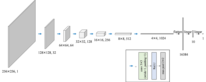
In this study, the tensile properties of tempered martensite steel were analyzed using a combination of an experimental approach and deep learning. The martensite steels were tempered in two stages, and fine and coarse cementite particles were mixed through two-stage tempering. The samples were heated to 923 and 973 K and held isothermally for 30, 45, and 60 min. They were then cooled to 723, 773, and 823 K; held isothermally for 30, 45, and 60 min; and furnace-cooled to room temperature (296 ± 2 K). The combination of low tempering temperature and short holding time in the first stage resulted in high tensile strength. When the tempering temperature at the first stage was 923 K, the combination of low tempering temperature and long holding time at the second stage resulted in high total elongation. This means that decreasing the number of coarse cementite particles and increasing the number of fine cementite particles improve the strength–ductility balance. Using the results obtained by the experimental approach, an image-based regression model was constructed that can accurately suggest the relationship between the microstructure and tensile properties of tempered martensite steel. We succeeded in developing image-based regression models with high accuracy using a convolutional neural network (CNN). Moreover, gradient-weighted class activation mapping (Grad-CAM) suggested that fine cementite particles and coarse and spheroidal cementite particles are the dominant factors for tensile strength and total elongation, respectively.

| [1] |
Nansai K, Watari T (2022) Innovative changes in material use for transition to a carbon-neutral society. Mater Cycles Waste Manag Res 33: 17–24. https://doi.org/10.3985/mcwmr.33.17 doi: 10.3985/mcwmr.33.17

|
| [2] |
Tsuchiyama T, Sakamoto T, Tanaka S, et al. (2020) Control of core-shell type second phase formed via interrupted quenching and intercritical annealing in a medium manganese steel. ISIJ Int 60: 2954–2962. https://doi.org/10.2355/isijinternational.ISIJINT-2020-164 doi: 10.2355/isijinternational.ISIJINT-2020-164
|
| [3] |
Kim JH, Kwon MH, Lee JS, et al. (2021) Influence of isothermal treatment prior to initial quenching of Q & P process on microstructure and mechanical properties of medium Mn steel. ISIJ Int 61: 518–526. https://doi.org/10.2355/isijinternational.ISIJINT-2019-733 doi: 10.2355/isijinternational.ISIJINT-2019-733
|
| [4] |
Okai D, Yae M, Yamamoto A, et al. (2017) EBSD observation of pure iron with near-cube orientation fabricated by cold rolling and annealing. Mater Trans 58: 838–841. https://doi.org/10.2320/matertrans.M2016443 doi: 10.2320/matertrans.M2016443
|
| [5] |
Okai D, Yamamoto A, DoiT, et al. (2021) Characteristics of cube orientation for pure iron tape fabricated by cold rolling and annealing. Mater Sci Forum 1016: 1830–1834. https://doi.org/10.4028/www.scientific.net/msf.1016.1830 doi: 10.4028/www.scientific.net/msf.1016.1830
|
| [6] | Liu CT, Gurland J (1968) The strengthening mechanism in spheroidized carbon steel. Trans TMS-AIME 242: 1535–1542. |
| [7] |
Ning J, Feng Y, Wang M, et al. (2017) Dependence of tensile properties on microstructural features of bimodal-sized ferrite/cementite steels. J Iron Steel Res Int 24: 67–76. https://doi.org/10.1016/S1006-706X(17)30010-9 doi: 10.1016/S1006-706X(17)30010-9
|
| [8] |
Tsuchida N, Ueji R, Gong W, et al. (2023) Stress partitioning between bcc and cementite phases discussed from phase stress and dislocation density in martensite steels. Scr Mater 222: 115002. https://doi.org/10.1016/j.scriptamat.2022.115002 doi: 10.1016/j.scriptamat.2022.115002
|
| [9] |
Hayakawa K, Ogawa T, He L, et al. (2024) Improvement in the strength–ductility balance of tempered martensite steel by controlling cementite particle size distribution. J Mater Eng Perform 33: 6675–6685. https://doi.org/10.1007/s11665-023-08428-w doi: 10.1007/s11665-023-08428-w
|
| [10] |
Wang Z, Ogawa T, Adachi Y (2019) Properties-to-microstructure-to-processing inverse analysis for steels via machine learning. ISIJ Int 59: 1691–1694. https://doi.org/10.2355/isijinternational.ISIJINT-2019-089 doi: 10.2355/isijinternational.ISIJINT-2019-089
|
| [11] |
Sawai K, Chen TT, Sun F, et al. (2024) Image regression analysis for linking the microstructure and property of steel. Results Mater 21: 100526. https://doi.org/10.1016/j.rinma.2023.100526 doi: 10.1016/j.rinma.2023.100526
|
| [12] |
Noguchi S, Wang H, Inoue J (2022) Identification of microstructures critically affecting material properties using machine learning framework based on met-allurgists' thinking process. Sci Rep 12: 14238. https://doi.org/10.1038/s41598-022-17614-0 doi: 10.1038/s41598-022-17614-0
|
| [13] |
Krizhevsky A, Sutskever I, Hinton GE (2017) ImageNet classification with deep convolutional neural networks. Commun ACM 60: 84–90. https://doi.org/10.1145/3065386 doi: 10.1145/3065386
|
| [14] |
Selvaraju RR, Cogswell M, Das A, et al. (2020) Grad-CAM: Visual explanations from deep networks via gradient-based localization. Int J Comput Vision 128: 336–359. https://doi.org/10.1007/s11263-019-01228-7 doi: 10.1007/s11263-019-01228-7
|
| [15] |
Liang JW, Shen YF, Misra RDK, et al. (2021) High strength-superplasticity combination of ultrafine-grained ferritic steel: the significant role of nanoscale carbides. J Mater Sci Technol 83: 131–144. https://doi.org/10.1016/j.jmst.2020.11.078 doi: 10.1016/j.jmst.2020.11.078
|


Figures(5)

Kengo Sawai, Keiya Sugiura, Toshio Ogawa, Ta-Te Chen, Fei Sun, Yoshitaka Adachi. Analysis of tensile properties in tempered martensite steels with different cementite particle size distributions[J]. AIMS Materials Science, 2024, 11(5): 1056-1064. doi: 10.3934/matersci.2024050


 DownLoad: