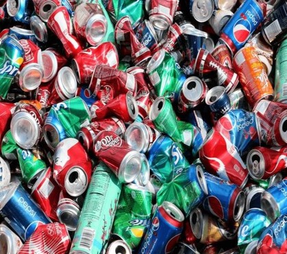
This study used rice husk ash to reinforce recycled aluminium waste cans matrix through stir casting technique to produce a composite. The rice husk ash was added to the aluminium matrix in 0, 5, 10, 15, and 20 wt%. Mechanical and microstructural analyses were carried out on the composites. The tensile strength of the composite increases at 5 wt% addition of reinforcement and increases further to reach a maximum of 121.6 MPa at 10 wt% addition. The tensile value then dropped at 15 wt% and reduced further at the 20 wt% particulate addition. A similar trend was observed for the impact strength with the maximum value of 81.5 J occurring at 10 wt% addition before declining at the higher percentages of reinforcement. The hardness of the composites continues to increase as the percentage of the rice husk addition rises leading to the highest Brinell hardness number (BHN) of 74.5 occurring at the highest percentage of rice husk ash addition. The density of the composites decreases as the wt% addition of the reinforcement increases giving the lowest density value of 2.46 g/cm3 at 20 wt% addition. The microstructures exhibited uniformity in the dispersion of the reinforcement into the aluminium matrix, although little particulate agglomeration could be noticed at higher percentages of rice husk addition. This study provides a significant boost to the attainment of lightweight materials in the automobile and other allied industries. The improvement in the mechanical properties and the lower density of the composites attained in this study are vital factors considered in material selection and design for lightweight engineering applications.
Citation: Olatunji P Abolusoro, Moshibudi Caroline Khoathane, Washington Washington. Mechanical and microstructural characteristics of recycled aluminium matrix reinforced with rice husk ash[J]. AIMS Materials Science, 2024, 11(5): 918-934. doi: 10.3934/matersci.2024044
This study used rice husk ash to reinforce recycled aluminium waste cans matrix through stir casting technique to produce a composite. The rice husk ash was added to the aluminium matrix in 0, 5, 10, 15, and 20 wt%. Mechanical and microstructural analyses were carried out on the composites. The tensile strength of the composite increases at 5 wt% addition of reinforcement and increases further to reach a maximum of 121.6 MPa at 10 wt% addition. The tensile value then dropped at 15 wt% and reduced further at the 20 wt% particulate addition. A similar trend was observed for the impact strength with the maximum value of 81.5 J occurring at 10 wt% addition before declining at the higher percentages of reinforcement. The hardness of the composites continues to increase as the percentage of the rice husk addition rises leading to the highest Brinell hardness number (BHN) of 74.5 occurring at the highest percentage of rice husk ash addition. The density of the composites decreases as the wt% addition of the reinforcement increases giving the lowest density value of 2.46 g/cm3 at 20 wt% addition. The microstructures exhibited uniformity in the dispersion of the reinforcement into the aluminium matrix, although little particulate agglomeration could be noticed at higher percentages of rice husk addition. This study provides a significant boost to the attainment of lightweight materials in the automobile and other allied industries. The improvement in the mechanical properties and the lower density of the composites attained in this study are vital factors considered in material selection and design for lightweight engineering applications.

| [1] | Patel M, Pardhi B, Chopara S, et al. (2008) Lightweight composite materials for automotive—A review. IRJET 5: 41–47. Available from: https://www.researchgate.net/publication/340646173_Lightweight_Composite_Materials_for_Automotive_-A_Review. |
| [2] | Jones RM (2015) Mechanics of Composite Materials, 2 Eds., New York: CRC Press, 1–52. https://doi.org/10.1201/9781498711067 |
| [3] |
Ikubanni PP, Oki M, Adeleke AA (2020) A review of ceramic/bio-based hybrid reinforced aluminium matrix composites. Cogent Eng 7: 1727167. https://doi.org/10.1080/23311916.2020.1727167 doi: 10.1080/23311916.2020.1727167

|
| [4] | Abolusoro OP, Akinlabi ET (2019) Wear and corrosion in friction stir welding of aluminium alloys—An overview. Int J Mech Prod Eng Res Dev 9: 967–982. Available from: https://www.researchgate.net/publication/333356596_Wear_and_Corrosion_Behaviour_of_Friction_Stir_Welded_Aluminium_Alloys-An_Overview. |
| [5] |
Shoag MD, Rahman MF (2021) Using recycling aluminum cans as composite materials aluminum fiber. IOP Conf Ser Earth Environ Sci 943: 012028. https://doi.org/10.1088/1755-1315/943/1/012028 doi: 10.1088/1755-1315/943/1/012028
|
| [6] |
Sharma AK, Bhandari R, Pinca-Bretotean C (2020) A systematic overview on fabrication aspects and methods of aluminium metal matrix composites. Mater Today Proc 45: 4133–4138. https://doi.org/10.1016/j.matpr.2020.11.899 doi: 10.1016/j.matpr.2020.11.899
|
| [7] |
Bahrami N, Soltani N, Pech-Canul MI, et al. (2016) Development of metal-matrix composites from industrial/agricultural waste materials and their derivatives. Crit Rev Environ Sci Technol 46: 143–208. https://doi.org/10.1080/10643389.2015.1077067 doi: 10.1080/10643389.2015.1077067
|
| [8] |
Kulkarni PP, Siddeswarappa B, Kariyappla SHK (2019) A survey on effect of agro-waste ash as reinforcement on aluminium base metal matrix composites. Open J Compos Mater 9: 12–26. https://doi.org/10.4236/ojcm.2019.93019 doi: 10.4236/ojcm.2019.93019
|
| [9] |
Olufunmilayo OJ, Kunle OB (2019) Agricultural waste as a reinforcement particulate for Al metal matrix composites (AMMCs). Rev MDPI Fibers 7: 7–33. https://doi.org/10.3390/fib7040033 doi: 10.3390/fib7040033
|
| [10] |
Jagannath V, Harish K (2019) Fly ash, rice husk ash as reinforcement with aluminium metal matrix composite: A review of technique, parameter and outcome. ICAPIE 2019: 953–962. https://doi.org/10.1007/978-981-15-8542-5_84 doi: 10.1007/978-981-15-8542-5_84
|
| [11] |
Yekinni AA, Durowoju MO, Agunsoye JO, et al. (2019) Automotive application of hybrid composites of aluminium alloy matrix: A review of rice husk ash-based reinforcements. Int J Compos Mater 9: 44–52. https://doi.org/10.5923/j.cmaterials.20190902.03 doi: 10.5923/j.cmaterials.20190902.03
|
| [12] |
Priyank D, Amit S (2022) Aluminum metal matrix composites reinforced with rice husk ash: A review. Mater Today Proc 62: 4194–4201. https://doi.org/10.1016/j.matpr.2022.04.711 doi: 10.1016/j.matpr.2022.04.711
|
| [13] | Alanemea KK, Adewale TM (2013) Influence of rice husk ash–silicon carbide weight ratio on the mechanical behavior of Al-Mg-Si alloy matrix hybrid composite. Tribol Indust 35: 163–172. Available from: https://www.researchgate.net/publication/281891199_Influence_of_Rice_Husk_Ash_-_Silicon_Carbide_Weight_Ratios_on_the_Mechanical_behaviour_of_Al-Mg-Si_Alloy_Matrix_Hybrid_Composites. |
| [14] |
Masoumeh K, Naser F, Pech-Canul MI, et al. (2024) Rice husk at a glance: From agro-industrial to modern applications. Rice Sci 31: 14–32. https://doi.org/10.1016/j.rsci.2023.08.005 doi: 10.1016/j.rsci.2023.08.005
|
| [15] |
Gadve RD, Trivedi Y, Sangal VK, et al. (2023) Utilization of rice husk ash as an effective reinforcement in polyether sulfone-based composites for printed circuit board. J Mater Sci Mater Electron 34: 1953. https://doi.org/10.1007/s10854-023-11367-w doi: 10.1007/s10854-023-11367-w
|
| [16] |
Mohd Joharudin NF, Abdul Latif N, Mustapa MS, et al. (2019) Effect of amorphous silica by rice husk ash on physical properties and microstructures of recycled aluminium chip AA7075. Materialwiss Werkstofftech 50: 283–288. https://doi.org/10.1002/mawe.201800229 doi: 10.1002/mawe.201800229
|
| [17] |
Ziada M, Erdem S, González-Lezcano AR, et al. (2023) Influence of various fibers on the physico-mechanical properties of a sustainable geopolymer mortar-based on metakaolin and slag. Eng Sci Technol Int J 46: 101501. https://doi.org/10.1016/j.jestch.2023.101501 doi: 10.1016/j.jestch.2023.101501
|
| [18] | Abolusoro OP, Orah AM, Yusuf AS, et al. (2023) Investigation of the energy capabilities of selected agricultural wastes in a fluidized-bed combustor. 2023 International Conference on Science, Engineering and Business for Sustainable Development Goals (SEB-SDG). https://doi.org/10.1109/SEB-SDG57117.2023.10124555 |
| [19] |
Saravanan SD, Kumar MS (2013) Effect of mechanical properties on rice husk ash reinforced aluminium alloy (AlSi10Mg) matrix composites. Proc Eng 64: 1505–1513. https://doi.org/10.1016/j.proeng.2013.09.232 doi: 10.1016/j.proeng.2013.09.232
|
| [20] |
Seikh Z, Sekh M, Kunar S, et al. (2022) Rice husk ash reinforced aluminium metal matrix composites: A review. Mat Sci Forum 1070: 55–70. https://doi.org/10.4028/p-u8s016 doi: 10.4028/p-u8s016
|
| [21] |
Darekar VS, Kulthe MG, Goyal A, et al. (2024) Rice husk ash: Effective reinforcement for epoxy-based composites for electronic applications. J Electron Mater 53: 1344–1359. https://doi.org/10.1007/s11664-023-10835-7 doi: 10.1007/s11664-023-10835-7
|
| [22] | Pratapa RY, Lakshmi NK, Kedar MM, et al. (2023) Characterisation of Al-6061-T6 metal matrix composites reinforced with rice husk ash and Bakelite powder. Mater Today Proc. https://doi.org/10.1016/j.matpr.2023.04.570 |
| [23] | Vasamsetti S, Dumpala L, Subbarao VV (2022) Effect of nano-rice husk ash reinforcement on the hardness of Al6061 using Taguchi method, In: Narasimham GSVL, Babu AV, Reddy SS, et al. Innovations in Mechanical Engineering. Lecture Notes in Mechanical Engineering, Singapore: Springer. https://doi.org/10.1007/978-981-16-7282-8_62 |
| [24] | Prasad DS, Rama KA (2011) Production and mechanical properties of A356.2/RHA composites. Int J of Adv Sci and Tech 33: 51–58. Available from: https://www.researchgate.net/publication/284651427_Production_and_Mechanical_Properties_of_A3562_RHA_Composites#fullTextFileContent. |
| [25] | ASTM (2015) Designation: B557−15 Standard Test Methods for Tension Testing Wrought and Cast Aluminum—ASTM International. 1–16. https://doi.org/10.1520/B0557-15.2 |
| [26] | ASTM E10-18 (2017) Standard Test Method for Brinell Hardness of Metallic Materials. Available from: https://www.astm.org/e0010-15a.html. |
| [27] | ASTM International Standard E23 of the year 2007. Test Methods for Notched Bar Impact Testing of Metallic Materials. |
| [28] |
Omoniyi P, Adekunle A, Ibitoye S, et al. (2022) Mechanical and microstructural evaluation of aluminium matrix composite reinforced with wood particles. J King Saud Univ–Eng Sci 34: 445–450. https://doi.org/10.1016/j.jksues.2021.01.006 doi: 10.1016/j.jksues.2021.01.006
|
| [29] |
Aigbodion VS, Hassan SB, Dauda ET, et al. (2010) The development of mathematical model for the prediction of ageing behaviour for Al-Cu-Mg/bagasse ash particulate composites. J Miner Mater Charact Eng 9: 907–917. https://doi.org/10.4236/jmmce.2010.910066 doi: 10.4236/jmmce.2010.910066
|
| [30] | Hamouda AMS, Sulaiman S, Vijayaram TR, et al. (2007) Processing and characterization of particulate reinforced aluminium silicon matrix composite. J Achiev Mater Manuf Eng 2: 11–16. Available from: https://www.researchgate.net/publication/40542990_Processing_and_characterisation_of_particulate_reinforced_aluminium_silicon_matrix_composite. |
| [31] | Aigbodion VS, Hassan SB, Dauda ET, et al. (2011) Experimental study of ageing behaviour of Al-Cu-Mg/bagasse ash particulate composites. Tribol Indust 33: 28–35. Available from: https://www.researchgate.net/publication/267979145_Experimental_Study_of_Ageing_Behaviour_of_Al-Cu-MgBagasse_Ash_Particulate_Composites. |
| [32] | Neelima DC, Mahesh V, Selvaraj N (2011) Mechanical characterization of aluminium silicon carbide composite. Int J Appl Eng Res 1: 793–799. Available from: https://www.scirp.org/reference/referencespapers?referenceid = 606668. |
| [33] |
Abdulwahab M, Umaru OB, Bawa MA, et al. (2017) Microstructural and thermal study of Al-Si-Mg/melon shell ash particulate composite. Results Phys 7: 947–954. https://doi.org/10.1016/j.rinp.2017.02.016 doi: 10.1016/j.rinp.2017.02.016
|
| [34] |
Suleiman IY, Salihu SA, Mohammed TA (2018) Investigation of mechanical, microstructure, and wear behaviours of Al-12%Si/reinforced with melon shell ash particulates. Int J Adv Manuf Technol 97: 4137–4144. https://doi.org/10.1007/s00170-018-2157-9 doi: 10.1007/s00170-018-2157-9
|
| [35] | Usman AM, Raji A, Waziri NH, et al. (2014) Aluminium alloy-rice husk ash composites production and analysis. Leonardo Electron J Pract Technol 25: 84–98. Available from: https://www.researchgate.net/publication/287933106_Aluminium_alloy_-_rice_husk_ash_composites_production_and_analysis |
| [36] | Aigbodion VS (2012) Development of Al-Si-Fe/rice husk ash particulate composites synthesis by double stir casting method. Usak Univ J Mat Sci 2: 187–197. https://dergipark.org.tr/en/pub/uujms/issue/13552/164155 |
| [37] | Shanmughasundaram P, Subramanian R, Prabhu G (2011) Some studies on aluminium-fly ash composites fabricated by two-step stir casting method. Eur J Sci Res 63: 204–218. Available from: https://www.researchgate.net/publication/267263404_Some_Studies_on_Aluminium_-_Fly_Ash_Composites_Fabricated_by_Two_Step_Stir_Casting_Method#fullTextFileContent. |
| [38] | Lingaraju D, Sreekanth GV (2014) Rice husk ash reinforced in aluminium matrix nanocomposite: A review. J Basic Appl Eng Res 1: 35–40. http://www.krishisanskriti.org/jbaer.html |
| [39] | Prasad DS, Krishna AR (2010) Fabrication and characterization of A356.2 RHA composite. Int J Eng Sci Technol 2: 7603–7608. Available from: https://www.researchgate.net/publication/285254345_Fabrication_and_Characterization_of_A3562-Rice_Husk_Ash_Composite_using_Stir_casting_technique. |
| [40] | Prasad DS, Krishna AR (2011) Production and mechanical properties of A356.2 RHA composite. Int J Adv Sci Technol 33: 51–58. Available from: http://article.nadiapub.com/IJAST/vol33/5.pdf. |
| [41] |
Omoniyi P, Abolusoro O, Olorunpomi O, et al. (2022) Corrosion properties of aluminum alloy reinforced with wood particles. J Compos Sci 6: 189. https://doi.org/10.3390/jcs6070189 doi: 10.3390/jcs6070189
|
| [42] |
Alaneme KK, Akintunde IB, Olubambi PA, et al. (2013) Fabrication characteristics and mechanical behaviour of rice husk ash–alumina reinforced Al-Mg-Si alloy matrix hybrid composites. J Mater Res Technol 2: 60–67. https://doi.org/10.1016/j.jmrt.2013.03.012 doi: 10.1016/j.jmrt.2013.03.012
|


Figures(11) / Tables(2)

Olatunji P Abolusoro, Moshibudi Caroline Khoathane, Washington Washington. Mechanical and microstructural characteristics of recycled aluminium matrix reinforced with rice husk ash[J]. AIMS Materials Science, 2024, 11(5): 918-934. doi: 10.3934/matersci.2024044


 DownLoad: