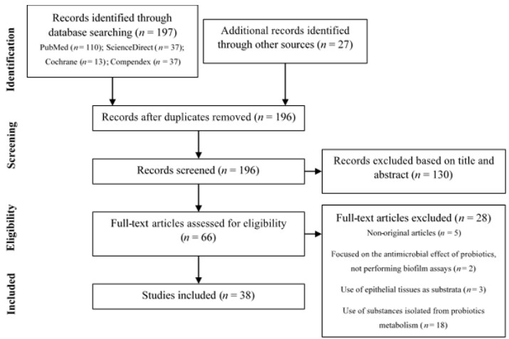
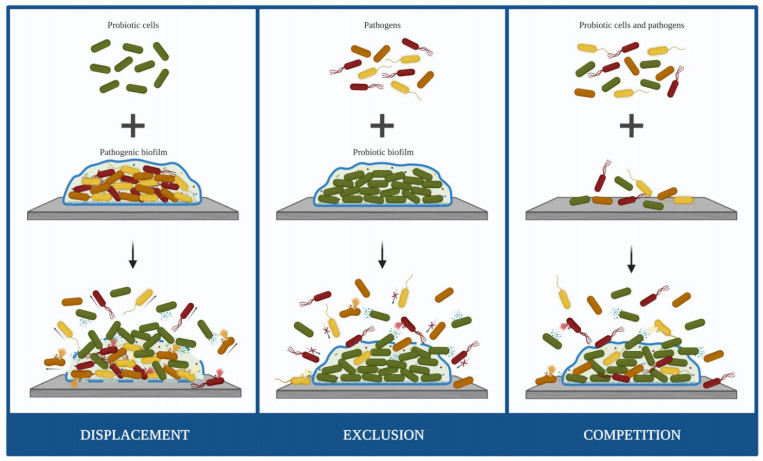
Biofilm-related infections are becoming a major clinical problem due to the increasingly widespread ability of pathogens to develop persistent biofilms in medical devices. The inadequate response of conventional antimicrobial strategies to counteract biofilm development demands urgent alternatives. An increasing interest in promoting a natural approach to health has intensified the research in the field of probiotics to battle pathogenic biofilms. This study aims to summarize the recent evidence supporting the effects of probiotic cells on the control and prevention of medical device-associated biofilms using a PRISMA-oriented (Preferred Reporting Items for Systematic reviews and Meta-Analyses) systematic search. This review demonstrated that probiotic cells have the potential to be used as biocontrol agents against biofilm formation by a broad spectrum of microorganisms. The restriction of biofilm growth caused by probiotics seemed to be strain-specific and independent of the antibiofilm strategy used (displacement, exclusion or competition). Lactobacillus, Lactococcus and Streptococcus were the most studied genus of probiotics and those with the higher capability to hinder biofilm formation, causing reductions up to 99.9%. These findings will pave the way to further experiments on the topic so that probiotic cells may become part of the clinical arsenal for the prevention and treatment of medical device-associated infections.
Citation: Fábio M. Carvalho, Rita Teixeira-Santos, Filipe J. M. Mergulhão, Luciana C. Gomes. Targeting biofilms in medical devices using probiotic cells: a systematic review[J]. AIMS Materials Science, 2021, 8(4): 501-523. doi: 10.3934/matersci.2021031
Biofilm-related infections are becoming a major clinical problem due to the increasingly widespread ability of pathogens to develop persistent biofilms in medical devices. The inadequate response of conventional antimicrobial strategies to counteract biofilm development demands urgent alternatives. An increasing interest in promoting a natural approach to health has intensified the research in the field of probiotics to battle pathogenic biofilms. This study aims to summarize the recent evidence supporting the effects of probiotic cells on the control and prevention of medical device-associated biofilms using a PRISMA-oriented (Preferred Reporting Items for Systematic reviews and Meta-Analyses) systematic search. This review demonstrated that probiotic cells have the potential to be used as biocontrol agents against biofilm formation by a broad spectrum of microorganisms. The restriction of biofilm growth caused by probiotics seemed to be strain-specific and independent of the antibiofilm strategy used (displacement, exclusion or competition). Lactobacillus, Lactococcus and Streptococcus were the most studied genus of probiotics and those with the higher capability to hinder biofilm formation, causing reductions up to 99.9%. These findings will pave the way to further experiments on the topic so that probiotic cells may become part of the clinical arsenal for the prevention and treatment of medical device-associated infections.

| [1] | Srivastava A, Chandra N, Kumar S (2019) The role of biofilms in medical devices and implants, Biofilms in Human Diseases: Treatment and Control, Springer, Cham, 151-165. |
| [2] |
Sun F, Qu F, Ling Y, et al. (2013) Biofilm-associated infections: Antibiotic resistance and novel therapeutic strategies. Future Microbiol 8: 877-886. doi: 10.2217/fmb.13.58

|
| [3] |
Khatoon Z, McTiernan CD, Suuronen EJ, et al. (2018) Bacterial biofilm formation on implantable devices and approaches to its treatment and prevention. Heliyon 4: e01067. doi: 10.1016/j.heliyon.2018.e01067
|
| [4] |
Percival SL, Suleman L, Vuotto C, et al. (2015) Healthcare-associated infections, medical devices and biofilms: Risk, tolerance and control. J Med Microbiol 64: 323-334. doi: 10.1099/jmm.0.000032
|
| [5] |
Van Epps JS, Younger JG (2016) Implantable device-related infection. Shock 46: 597-608. doi: 10.1097/SHK.0000000000000692
|
| [6] | Tunney MM, Gorman SP, Patrick S (2002) Infection associated with medical devices. Int J Gen Syst 31: 195-205. |
| [7] |
Donlan RM (2001) Biofilms and device-associated infections. Emerg Infect Dis 7: 277-281. doi: 10.3201/eid0702.010226
|
| [8] |
Vertes A, Hitchins V, Phillips KS (2012) Analytical challenges of microbial biofilms on medical devices. Anal Chem 84: 3858-3866. doi: 10.1021/ac2029997
|
| [9] |
Veerachamy S, Yarlagadda T, Manivasagam G, et al. (2014) Bacterial adherence and biofilm formation on medical implants: A review. P I Mech Eng H 228: 1083-1099. doi: 10.1177/0954411914556137
|
| [10] |
Ramstedt M, Ribeiro IAC, Bujdakova H, et al. (2019) Evaluating efficacy of antimicrobial and antifouling materials for urinary tract medical devices: Challenges and recommendations. Macromol Biosci 19: e1800384. doi: 10.1002/mabi.201800384
|
| [11] |
Reid G (1999) Biofilms in infectious disease and on medical devices. Int J Antimicrob Ag 11: 223-226. doi: 10.1016/S0924-8579(99)00020-5
|
| [12] |
Bryers JD (2008) Medical biofilms. Biotechnol Bioeng 100: 1-18. doi: 10.1002/bit.21838
|
| [13] |
Darouiche RO (2004) Treatment of infections associated with surgical implants. N Engl J Med 350: 1422-1429. doi: 10.1056/NEJMra035415
|
| [14] |
Darouiche RO (2001) Device-associated infections: A macroproblem that starts with microadherence. Clin Infect Dis 33: 1567-1572. doi: 10.1086/323130
|
| [15] |
Campoccia D, Montanaro L, Arciola CR (2006) The significance of infection related to orthopedic devices and issues of antibiotic resistance. Biomaterials 27: 2331-2339. doi: 10.1016/j.biomaterials.2005.11.044
|
| [16] |
Azevedo AS, Almeida C, Melo LF, et al. (2017) Impact of polymicrobial biofilms in catheter-associated urinary tract infections. Crit Rev Microbiol 43: 423-439. doi: 10.1080/1040841X.2016.1240656
|
| [17] | World Health Organization, Report on the Burden of Endemic Health Care-Associated Infection Worldwide, 2011. Available from: https://apps.who.int/iris/bitstream/handle/10665/80135/9789241501507_eng.pdf;jsessionid=C2A2CD7A9910C3B4AC1FC3B18F1DBD11?sequence=1. |
| [18] |
Feneley RCL, Hopley IB, Wells PNT (2015) Urinary catheters: History, current status, adverse events and research agenda. J Med Eng Technol 39: 459-470. doi: 10.3109/03091902.2015.1085600
|
| [19] |
Flemming HC, Wingender J (2010) The biofilm matrix. Nat Rev Microbiol 8: 623-633. doi: 10.1038/nrmicro2415
|
| [20] |
Rabin N, Zheng Y, Opoku-Temeng C, et al. (2015) Biofilm formation mechanisms and targets for developing antibiofilm agents. Future Med Chem 7: 493-512. doi: 10.4155/fmc.15.6
|
| [21] |
Deva AK, Adams WP, Vickery K (2013) The role of bacterial biofilms in device-associated infection. Plast Reconstr Surg 132: 1319-1328. doi: 10.1097/PRS.0b013e3182a3c105
|
| [22] |
Garrett TR, Bhakoo M, Zhang Z (2008) Bacterial adhesion and biofilms on surfaces. Prog Nat Sci 18: 1049-1056. doi: 10.1016/j.pnsc.2008.04.001
|
| [23] |
Lindsay D, von Holy A (2006) Bacterial biofilms within the clinical setting: What healthcare professionals should know. J Hosp Infect 64: 313-325. doi: 10.1016/j.jhin.2006.06.028
|
| [24] |
Corte L, Pierantoni DC, Tascini C, et al. (2019) Biofilm specific activity: A measure to quantify microbial biofilm. Microorganisms 7: 73. doi: 10.3390/microorganisms7030073
|
| [25] | Marić S, Vraneš J (2007) Characteristics and significance of microbial biofilm formation. Period Biol 109: 115-121. |
| [26] |
Donlan RM (2002) Biofilms: Microbial life on surfaces. Emerg Infect Dis 8: 881-890. doi: 10.3201/eid0809.020063
|
| [27] | Vasudevan R (2014) Biofilms: Microbial cities of scientific significance. J Microbiol Exp 1: 84-98. |
| [28] | Floyd KA, Eberly AR, Hadjifrangiskou M (2017) Adhesion of bacteria to surfaces and biofilm formation on medical devices, Biofilms and Implantable Medical Devices: Infection and Control, Woodhead Publishing, 47-95. |
| [29] |
Chen M, Yu Q, Sun H (2013) Novel strategies for the prevention and treatment of biofilm related infections. Int J Mol Sci 14: 18488-18501. doi: 10.3390/ijms140918488
|
| [30] |
Zhu Z, Wang Z, Li S, et al. (2019) Antimicrobial strategies for urinary catheters. J Biomed Mater Res A 107: 445-467. doi: 10.1002/jbm.a.36561
|
| [31] | Dwivedi P, Narvi SS, Tewari RP (2013) Application of polymer nanocomposites in the nanomedicine landscape: Envisaging strategies to combat implant associated infections. J Appl Biomater Funct Mater 11: 129-142. |
| [32] |
Singha P, Locklin J, Handa H (2017) A review of the recent advances in antimicrobial coatings for urinary catheters. Acta Biomater 50: 20-40. doi: 10.1016/j.actbio.2016.11.070
|
| [33] |
Prabhurajeshwar C, Chandrakanth RK (2017) Probiotic potential of lactobacilli with antagonistic activity against pathogenic strains: An in vitro validation for the production of inhibitory substances. Biomed J 40: 270-283. doi: 10.1016/j.bj.2017.06.008
|
| [34] |
de Melo Pereira GV, de Oliveira Coelho B, Magalhães Júnior AI, et al. (2018) How to select a probiotic? A review and update of methods and criteria. Biotechnol Adv 36: 2060-2076. doi: 10.1016/j.biotechadv.2018.09.003
|
| [35] |
Radaic A, Ye C, Parks B, et al. (2020) Modulation of pathogenic oral biofilms towards health with nisin probiotic. J Oral Microbiol 12: 1809302. doi: 10.1080/20002297.2020.1809302
|
| [36] | FAO (2006) Probiotics in food: Health and nutritional properties and guidelines for evaluation, 2006. Available from: http://www.fao.org/3/a-a0512e.pdf. |
| [37] | Carvalho FM, Teixeira-Santos R, Mergulhão FJM, et al. (2021) The use of probiotics to fight biofilms in medical devices: A systematic review and meta-analysis. Microorganisms 9: 1-26. |
| [38] |
Barzegari A, Kheyrolahzadeh K, Mahdi S, et al. (2020) The battle of probiotics and their derivatives against biofilms. Infect Drug Resist 13: 659-672. doi: 10.2147/IDR.S232982
|
| [39] |
Reid G (1999) The scientific basis for probiotic strains of Lactobacillus. Appl Environ Microb 65: 3763-3766. doi: 10.1128/AEM.65.9.3763-3766.1999
|
| [40] |
Markowiak P, Ślizewska K (2017) Effects of probiotics, prebiotics, and synbiotics on human health. Nutrients 9: 1021. doi: 10.3390/nu9091021
|
| [41] |
Suez J, Zmora N, Segal E, et al. (2019) The pros, cons, and many unknowns of probiotics. Nat Med 25: 716-729. doi: 10.1038/s41591-019-0439-x
|
| [42] |
Salas-Jara M, Ilabaca A, Vega M, et al. (2016) Biofilm forming Lactobacillus: New challenges for the development of probiotics. Microorganisms 4: 35. doi: 10.3390/microorganisms4030035
|
| [43] |
Saxelin M, Tynkkynen S, Mattila-Sandholm T, et al. (2005) Probiotic and other functional microbes: From markets to mechanisms. Curr Opin Biotech 16: 204-211. doi: 10.1016/j.copbio.2005.02.003
|
| [44] | Fioramonti J, Theodorou V, Bueno L (2003) Probiotics: What are they? What are their effects on gut physiology? Best Pract Res Cl Ga 17: 711-724. |
| [45] |
Gogineni VK, Morrow LE (2013) Probiotics: Mechanisms of action and clinical applications. J Prob Health 1: 1-11. doi: 10.4172/2329-8901.1000101
|
| [46] |
Hemaiswarya S, Raja R, Ravikumar R, et al. (2013) Mechanism of action of probiotics. Braz Arch Biol Techn 56: 113-119. doi: 10.1590/S1516-89132013000100015
|
| [47] | Khalighi A, Behdani R, Kouhestani S (2016) Probiotics: A comprehensive review of their classification, mode of action and role in human nutrition, In: Rao V, Rao L, Probiotics and Prebiotics in Human Nutrition and Health, Croatia: InTech, 10: 63646. |
| [48] |
Moher D, Liberati A, Tetzlaff J, et al. (2009) Preferred reporting items for systematic reviews and meta-analyses: The PRISMA statement. Plos Med 6: e1000097. doi: 10.1371/journal.pmed.1000097
|
| [49] | Nemcová R (1997) Criteria for selection of lactobacilli for probiotic use. Vet Med 42: 19-27. |
| [50] |
Kim AR, Ahn KB, Yun CH, et al. (2019) Lactobacillus plantarum lipoteichoic acid inhibits oral multispecies biofilm. J Endod 45: 310-315. doi: 10.1016/j.joen.2018.12.007
|
| [51] |
Bermudez-Brito M, Plaza-Díaz J, Muñoz-Quezada S, et al. (2012) Probiotic mechanisms of action. Ann Nutr Metab 61: 160-174. doi: 10.1159/000342079
|
| [52] |
Muñoz M, Mosquera A, Alméciga-Díaz CJ, et al. (2012) Fructooligosaccharides metabolism and effect on bacteriocin production in Lactobacillus strains isolated from ensiled corn and molasses. Anaerobe 18: 321-330. doi: 10.1016/j.anaerobe.2012.01.007
|
| [53] |
Kechagia M, Basoulis D, Konstantopoulou S, et al. (2013) Health benefits of probiotics: A review. ISRN Nutr 2013: 481651. doi: 10.5402/2013/481651
|
| [54] |
Holzapfel WH, Haberer P, Geisen R, et al. (2001) Taxonomy and important features of probiotic microorganisms in food and nutrition. Am J Clin Nutr 73: 365-373. doi: 10.1093/ajcn/73.2.365s
|
| [55] |
Carr FJ, Chill D, Maida N (2002) The lactic acid bacteria: A literature survey. Crit Rev Microbiol 28: 281-370. doi: 10.1080/1040-840291046759
|
| [56] |
Leroy F, De Vuyst L (2004) Lactic acid bacteria as functional starter cultures for the food fermentation industry. Trends Food Sci Tech 15: 67-78. doi: 10.1016/j.tifs.2003.09.004
|
| [57] |
Ng SC, Hart AL, Kamm MA, et al. (2009) Mechanisms of action of probiotics: Recent advances. Inflamm Bowel Dis 15: 300-310. doi: 10.1002/ibd.20602
|
| [58] | Chen Q, Zhu Z, Wang J, et al. (2017) Probiotic E. coli Nissle 1917 biofilms on silicone substrates for bacterial interference against pathogen colonization. Acta Biomater 50: 353-360. |
| [59] | Maldonado NC, Silva De Ruiz C, Cecilia M, et al. (2007) A simple technique to detect Klebsiella biofilm-forming-strains. Inhibitory potential of Lactobacillus fermentum CRL 1058 whole cells and products, In: Méndez-Vilas A, Communicating Current Research and Educational Topics and Trends in Applied Microbiology, Formatex, 52-59. |
| [60] |
McMillan A, Dell M, Zellar MP, et al. (2011) Disruption of urogenital biofilms by lactobacilli. Colloid Surface B 86: 58-64. doi: 10.1016/j.colsurfb.2011.03.016
|
| [61] |
Velraeds MMC, van Belt-Gritter B De, Busscher HJ, et al. (2000) Inhibition of uropathogenic biofilm growth on silicone rubber in human urine by lactobacilli—A teleologic approach. World J Urol 18: 422-426. doi: 10.1007/PL00007084
|
| [62] |
Reid G, Tieszer C (1994) Use of lactobacilli to reduce the adhesion of Staphylococcus aureus to catheters. Int Biodeter Biodegr 34: 73-83. doi: 10.1016/0964-8305(95)00011-9
|
| [63] | Millsap K, Reid G, van der Mei HC, et al. (1994) Displacement of Enterococcus faecalis from hydrophobic and hydrophilic substrata by Lactobacillus and Streptococcus spp. as studied in a parallel plate flow chamber. Appl Environ Microb 60: 1867-1874. |
| [64] |
Ifeoma ME, Jennifer UK (2016) Inhibition of biofilms on urinary catheters using immobilized Lactobacillus cells. African J Microbiol Res 10: 920-929. doi: 10.5897/AJMR2016.8056
|
| [65] |
Derakhshandeh S, Shahrokhi N, Khalaj V, et al. (2020) Surface display of uropathogenic Escherichia coli FimH in Lactococcus lactis: In vitro characterization of recombinant bacteria and its protectivity in animal model. Microb Pathogensis 141: 103974. doi: 10.1016/j.micpath.2020.103974
|
| [66] | Busscher HJ, van Hoogmoed CG, Geertsema-Doornbusch GI, et al. (1997) Streptococcus thermophilus and its biosurfactants inhibit adhesion by Candida spp. on silicone rubber. Appl Environ Microb 63: 3810-3817. |
| [67] |
van der Mei HC, van de Belt-Gritter B, van Weissenbruch R, et al. (1999) Effect of consumption of dairy products with probiotic bacteria on biofilm formation on silicone rubber implant surfaces in an artificial throat. Food Bioprod Process 77: 156-158. doi: 10.1205/096030899532303
|
| [68] |
van der Mei HC, Free RH, Elving GJ, et al. (2000) Effect of probiotic bacteria on prevalence of yeasts in oropharyngeal biofilms on silicone rubber voice prostheses in vitro. J Med Microbiol 49: 713-718. doi: 10.1099/0022-1317-49-8-713
|
| [69] |
van der Mei HC, Buijssen KJDA, van der Laan BFAM, et al. (2014) Voice prosthetic biofilm formation and Candida morphogenic conversions in absence and presence of different bacterial strains and species on silicone-rubber. Plos One 9: e104508. doi: 10.1371/journal.pone.0104508
|
| [70] |
Jiang Q, Stamatova I, Kainulainen V, et al. (2016) Interactions between Lactobacillus rhamnosus GG and oral micro-organisms in an in vitro biofilm model. BMC Microbiol 16: 149. doi: 10.1186/s12866-016-0759-7
|
| [71] |
Kang MS, Oh JS, Lee HC, et al. (2011) Inhibitory effect of Lactobacillus reuteri on periodontopathic and cariogenic bacteria. J Microbiol 49: 193-199. doi: 10.1007/s12275-011-0252-9
|
| [72] |
Teanpaisan R, Piwat S, Dahlén G (2011) Inhibitory effect of oral Lactobacillus against oral pathogens. Lett Appl Microbiol 53: 452-459. doi: 10.1111/j.1472-765X.2011.03132.x
|
| [73] | Marttinen AM, Haukioja AL, Keskin M, et al. (2013) Effects of Lactobacillus reuteri PTA 5289 and L. paracasei DSMZ16671 on the adhesion and biofilm formation of Streptococcus mutans. Curr Microbiol 67: 193-199. |
| [74] |
Söderling EM, Marttinen AM, Haukioja AL (2011) Probiotic lactobacilli interfere with Streptococcus mutans biofilm formation in vitro. Curr Microbiol 62: 618-622. doi: 10.1007/s00284-010-9752-9
|
| [75] |
Lee SH, Kim YJ (2014) A comparative study of the effect of probiotics on cariogenic biofilm model for preventing dental caries. Arch Microbiol 196: 601-609. doi: 10.1007/s00203-014-0998-7
|
| [76] |
Jaffar N, Ishikawa Y, Mizuno K, et al. (2016) Mature biofilm degradation by potential probiotics: Aggregatibacter actinomycetemcomitans versus Lactobacillus spp. Plos One 11: e0159466. doi: 10.1371/journal.pone.0159466
|
| [77] | Vilela SFG, Barbosa JO, Rossoni RD, et al. (2015) Lactobacillus acidophilus ATCC 4356 inhibits biofilm formation by C. albicans and attenuates the experimental candidiasis in Galleria mellonella. Virulence 6: 29-39. |
| [78] |
Krzyściak W, Kościelniak D, Papież M, et al. (2017) Effect of a Lactobacillus salivarius probiotic on a double-species Streptococcus mutans and Candida albicans caries biofilm. Nutrients 9: 1242. doi: 10.3390/nu9111242
|
| [79] |
Rossoni RD, de Barros PP, de Alvarenga JA, et al. (2018) Antifungal activity of clinical Lactobacillus strains against Candida albicans biofilms: Identification of potential probiotic candidates to prevent oral candidiasis. Biofouling 34: 212-225. doi: 10.1080/08927014.2018.1425402
|
| [80] |
Lin X, Chen X, Tu Y, et al. (2017) Effect of probiotic lactobacilli on the growth of Streptococcus mutans and multispecies biofilms isolated from children with active caries. Med Sci Monit 23: 4175-4181. doi: 10.12659/MSM.902237
|
| [81] |
Song YG, Lee SH (2017) Inhibitory effects of Lactobacillus rhamnosus and Lactobacillus casei on Candida biofilm of denture surface. Arch Oral Biol 76: 1-6. doi: 10.1016/j.archoralbio.2016.12.014
|
| [82] | Ciandrini E, Campana R, Baffone W (2017) Live and heat-killed Lactobacillus spp. interfere with Streptococcus mutans and Streptococcus oralis during biofilm development on titanium surface. Arch Oral Biol 78: 48-57. |
| [83] |
Comelli EM, Guggenheim B, Stingele F, et al. (2002) Selection of dairy bacterial strains as probiotics for oral health. Eur J Oral Sci 110: 218-224. doi: 10.1034/j.1600-0447.2002.21216.x
|
| [84] |
James KM, MacDonald KW, Chanyi RM, et al. (2016) Inhibition of Candida albicans biofilm formation and modulation of gene expression by probiotic cells and supernatant. J Med Microbiol 65: 328-336. doi: 10.1099/jmm.0.000226
|
| [85] |
Fernández CE, Giacaman RA, Tenuta LM, et al. (2015) Effect of the probiotic Lactobacillus rhamnosus LB21 on the cariogenicity of Streptococcus mutans UA159 in a dual-species biofilm model. Caries Res 49: 583-590. doi: 10.1159/000439315
|
| [86] |
Wu CC, Lin CT, Wu CY, et al. (2015) Inhibitory effect of Lactobacillus salivarius on Streptococcus mutans biofilm formation. Mol Oral Microbiol 30: 16-26. doi: 10.1111/omi.12063
|
| [87] |
Tahmourespour A, Kermanshahi RK (2011) The effect of a probiotic strain (Lactobacillus acidophilus) on the plaque formation of oral streptococci. Bosn J Basic Med Sci 11: 37-40. doi: 10.17305/bjbms.2011.2621
|
| [88] |
Vacca C, Contu MP, Rossi C, et al. (2020) In vitro interactions between Streptococcus intermedius and Streptococcus salivarius K12 on a titanium cylindrical surface. Pathogens 9: 1069. doi: 10.3390/pathogens9121069
|
| [89] | Fang K, Jin X, Hong SH (2018) Probiotic Escherichia coli inhibits biofilm formation of pathogenic E. coli via extracellular activity of DegP. Sci Rep 8: 4939. |
| [90] |
Hancock V, Dahl M, Klemm P (2010) Probiotic Escherichia coli strain Nissle 1917 outcompetes intestinal pathogens during biofilm formation. J Med Microbiol 59: 392-399. doi: 10.1099/jmm.0.008672-0
|
| [91] | Kıvanç M, Er S (2020) Biofilm formation of Candida spp. isolated from the vagina and antibiofilm activities of lactic acid bacteria on the these Candida isolates. Afr Health Sci 20: 641-648. |
| [92] |
Matsubara VH, Wang Y, Bandara HMHN, et al. (2016) Probiotic lactobacilli inhibit early stages of Candida albicans biofilm development by reducing their growth, cell adhesion, and filamentation. Appl Microbiol Biot 100: 6415-6426. doi: 10.1007/s00253-016-7527-3
|
| [93] | Alexandre Y, Le Berre R, Barbier G, et al. (2014) Screening of Lactobacillus spp. for the prevention of Pseudomonas aeruginosa pulmonary infections. BMC Microbiol 14: 107. |
| [94] |
Song H, Zhang J, Qu J, et al. (2019) Lactobacillus rhamnosus GG microcapsules inhibit Escherichia coli biofilm formation in coculture. Biotechnol Lett 41: 1007-1014. doi: 10.1007/s10529-019-02694-2
|
| [95] |
Sambanthamoorthy K, Feng X, Patel R, et al. (2014) Antimicrobial and antibiofilm potential of biosurfactants isolated from lactobacilli against multi-drug-resistant pathogens. BMC Microbiol 14: 197. doi: 10.1186/1471-2180-14-197
|
| [96] |
Kaur S, Sharma P, Kalia N, et al. (2018) Anti-biofilm properties of the fecal probiotic lactobacilli against Vibrio spp. Front Cell Infect Mi 8: 120. doi: 10.3389/fcimb.2018.00120
|
| [97] |
Otero MC, Nader-Macías ME (2006) Inhibition of Staphylococcus aureus by H2O2-producing Lactobacillus gasseri isolated from the vaginal tract of cattle. Anim Reprod Sci 96: 35-46. doi: 10.1016/j.anireprosci.2005.11.004
|
| [98] |
Azeredo J, Azevedo NF, Briandet R, et al. (2017) Critical review on biofilm methods. Crit Rev Microbiol 43: 313-351. doi: 10.1080/1040841X.2016.1208146
|
| [99] | Gomes M, Gomes LC, Santos RT, et al. (2020) PDMS in urinary tract devices: Applications, problems and potential solutions, In: Carlsen PN, 1st Ed, Polydimethylsiloxane: Structure and Applications, Nova Science Publishers. |
| [100] |
Khan F, Tabassum N, Kim YM (2020) A strategy to control colonization of pathogens: Embedding of lactic acid bacteria on the surface of urinary catheter. Appl Microbiol Biot 104: 9053-9066. doi: 10.1007/s00253-020-10903-6
|
| [101] |
Zhu Z, Yu F, Chen H, et al. (2017) Coating of silicone with mannoside-PAMAM dendrimers to enhance formation of non-pathogenic Escherichia coli biofilms against colonization of uropathogens. Acta Biomater 64: 200-210. doi: 10.1016/j.actbio.2017.10.008
|
| [102] |
Lopez AI, Kumar A, Planas MR, et al. (2011) Biomaterials biofunctionalization of silicone polymers using poly(amidoamine) dendrimers and a mannose derivative for prolonged interference against pathogen colonization. Biomaterials 32: 4336-4346. doi: 10.1016/j.biomaterials.2011.02.056
|
| [103] |
Gross G, van Der Meulen J, Snel J, et al. (2008) Mannose-specific interaction of Lactobacillus plantarum with porcine jejunal epithelium. FEMS Immunol Med Mic 54: 215-223. doi: 10.1111/j.1574-695X.2008.00466.x
|
| [104] |
Barth KA, Coullerez G, Nilsson LM, et al. (2008) An engineered mannoside presenting platform: Escherichia coli adhesion under static and dynamic conditions. Adv Funct Mater 18: 1459-1469. doi: 10.1002/adfm.200701246
|
| [105] | Tan L, Fu J, Feng F, et al. (2020) Engineered probiotics biofilm enhances osseointegration via immunoregulation and anti-infection. Sci Adv 6: eaba5723. |
| [106] |
Piqué N, Berlanga M, Miñana-Galbis D (2019) Health benefits of heat-killed (Tyndallized) probiotics: An overview. Int J Mol Sci 20: 2534. doi: 10.3390/ijms20102534
|
Figures(2) / Tables(2)

Fábio M. Carvalho, Rita Teixeira-Santos, Filipe J. M. Mergulhão, Luciana C. Gomes. Targeting biofilms in medical devices using probiotic cells: a systematic review[J]. AIMS Materials Science, 2021, 8(4): 501-523. doi: 10.3934/matersci.2021031


 DownLoad: