Citation: Stephan A. Brinckmann, Nishant Lakhera, Chris M. Laursen, Christopher Yakacki, Carl P. Frick. Characterization of poly(para-phenylene)-MWCNT solvent-cast composites[J]. AIMS Materials Science, 2018, 5(2): 301-319. doi: 10.3934/matersci.2018.2.301
| [1] | Mohammad Na'aim Abd Rahim, Mohd Shukor Salleh, Saifudin Hafiz Yahaya, Sivarao Subramonian, Azrin Hani Abdul Rashid, Syarifah Nur Aqida Syed Ahmad, Salah Salman Al-Zubaidi . Microstructural investigation and mechanical properties of Al2O3-MWCNTs reinforced aluminium composite. AIMS Materials Science, 2025, 12(2): 318-335. doi: 10.3934/matersci.2025017 |
| [2] | Ahmed Ali Farhan Ogaili, Ehsan S. Al-Ameen, Mohammed Salman Kadhim, Muhanad Nazar Mustafa . Evaluation of mechanical and electrical properties of GFRP composite strengthened with hybrid nanomaterial fillers. AIMS Materials Science, 2020, 7(1): 93-102. doi: 10.3934/matersci.2020.1.93 |
| [3] | Dorel Feldman . Poly(vinyl alcohol) nanocomposites: Recent contributions to engineering and medicine. AIMS Materials Science, 2021, 8(1): 119-129. doi: 10.3934/matersci.2021008 |
| [4] | Harikrishnan Pulikkalparambil, Jyotishkumar Parameswaranpillai, Jinu Jacob George, Krittirash Yorseng, Suchart Siengchin . Physical and thermo-mechanical properties of bionano reinforced poly(butylene adipate-co-terephthalate), hemp/CNF/Ag-NPs composites. AIMS Materials Science, 2017, 4(3): 814-831. doi: 10.3934/matersci.2017.3.814 |
| [5] | Hendra Suherman, Irmayani . Optimization of compression moulding parameters of multiwall carbon nanotube/synthetic graphite/epoxy nanocomposites with respect to electrical conductivity. AIMS Materials Science, 2019, 6(4): 621-634. doi: 10.3934/matersci.2019.4.621 |
| [6] | Chunyi Tang, Matthew Mullen, William B. Euler . Influence of solvent and molecular weight in wrinkle formation in spin-cast polystyrene thin films. AIMS Materials Science, 2020, 7(1): 60-74. doi: 10.3934/matersci.2020.1.60 |
| [7] | Neerajkumar Wayzode, Vinod Suryawanshi . Mechanical properties of graphene nanoplatelets reinforced glass/epoxy composites manufactured using resin film infusion process. AIMS Materials Science, 2023, 10(4): 693-709. doi: 10.3934/matersci.2023038 |
| [8] | Wisawat Keaswejjareansuk, Xiang Wang, Richard D. Sisson, Jianyu Liang . Electrospinning process control for fiber-structured poly(Bisphenol A-co-Epichlorohydrin) membrane. AIMS Materials Science, 2020, 7(2): 130-143. doi: 10.3934/matersci.2020.2.130 |
| [9] | Thomas J. Lee, Andrew H. Morgenstern, Thomas A. Höft, Brittany B. Nelson-Cheeseman . Dispersion of particulate in solvent cast magnetic thermoplastic polyurethane elastomer composites. AIMS Materials Science, 2019, 6(3): 354-362. doi: 10.3934/matersci.2019.3.354 |
| [10] | Huda A. Al-Salihi, Hadia Kadhim Judran . Effect of Al2O3 reinforcement nanoparticles on the tribological behaviour and mechanical properties of Al6061 alloy. AIMS Materials Science, 2020, 7(4): 486-498. doi: 10.3934/matersci.2020.4.486 |
Poly(para-phenylene) (PPP) has been shown to exhibit high tensile stiffness and strength values. Depending on the specific side chains present, tensile elastic modulus values range from 5 to 9 GPa, and yield strengths vary between 120 to 200 MPa [1,2,3,4]. The high strength of this polymer system is associated with the repeating aromatic phenyl rings in the backbone structure [4]; PPP has been explicitly noted as one of the strongest unreinforced polymers available [2]. In addition to high strength, PPP has several other favorable properties, which include good thermal stability [2], scratch resistance [3], biocompatibility [4,5,6], and shape-memory properties [7].
For typical PPP processing, temperatures upwards of 320 ℃ must be employed in fabrication methods such as pressing or injection molding [5,8,9]. This is characteristic of other aromatic polymers as well, such as commercially available polyphenylene sulfide (PPS) [10,11,12] and polyetheretherketone (PEEK) [13,14,15]. Despite the high temperatures required for fabrication, alternative solvent-casting techniques for PPS or PEEK are not typically utilized because they are insoluble in most solvents, with the exception of strong acids [16,17,18]. To the authors' knowledge, no studies have investigated the material properties of solvent-cast PPP, in spite of interest in manipulating the chemistry of PPP to improve solubility behavior [19,20].
Due to the convenience and ease of casting, which can be prepared in ambient conditions, solvent-casting is an advantageous technique for creating PPP films or coatings. Combining this manufacturing advantage with the beneficial properties of PPP, solvent-casting could be an effective way of creating biocompatible surfaces with robust tribological properties. For example, a potential orthopedic implant with high promise made from PPP has been previously investigated, however it required high compression molding techniques for manufacturing [4,5]. Furthermore, the ability to solvent-cast PPP opens new doors for polymer matrix composites by allowing for inclusion of reinforcements into a liquid PPP matrix during manufacturing.
Carbon nanotubes (CNTs) have frequently been considered as reinforcement for polymer-matrix composites [14,21,22] due to CNT's theoretical elastic modulus values on the order of 1 TPa and tensile strengths in excess of 50 GPa [23]. In addition to the mechanical properties, CNTs have excellent electrical and thermal properties [24]. Unfortunately, CNT reinforced polymers do not typically reach theoretical material properties [25]. This disparity between theoretical and empirical values may be due to the weak interfacial bonding between CNTs and their polymer matrix [26,27,28]. Conventional theories for composite behavior dictate that for load transfer from the matrix to the reinforcement, the adhesion properties between the reinforcement and matrix must be relatively strong; this is also the case with CNT composites [29]. Weak adhesion likely results in debonding of the reinforcement from the matrix, leading to premature crack nucleation and fracture. In addition, CNTs tend to aggregate due to secondary bonding of van der Waals forces [30], preventing good physical contact with the matrix. CNT agglomerations have been associated with negative impact on composite mechanical properties [24,31,32,33,34,35,36].
In an effort to increase the dispersion of CNTs within the polymer matrix, surface modified CNTs have been developed [37,38]. These functionalization techniques aid in the nanotube dispersion as well as increase the strength of the interface between CNTs and polymer matrices [39]. Several functionalization techniques, however, can disrupt the covalent bonding of the CNTs, creating a significant flaw in the tube which will severely weaken the theoretical strength of the material [24,31]. Using multi-walled carbon nanotubes (MWCNTs) can allow for functionalization of the exterior tube to facilitate dispersion, while maintaining mechanical properties of the inner tubes. Functionalized MWCNT-polymer composites have shown to blend the desirable properties of CNTs with polymer matrices [24,31,40] and PPP-MWCNT composites have been previously studied resulting in a favorable increase of the mechanical properties adding to the already strong and stiff polymer [41,42]. With successful creation of PPP-MWCNT composites, stiff wear resistant materials can be manufactured along with the possibility of tailoring shape memory transition temperatures for targeted uses, such as in the biomedical field.
In this study, a methodology for solvent-casting fabrication of thin film PPP and PPP-MWCNT composites is established. The properties of solvent-cast PPP are investigated first as a baseline, as solvent-casting of PPP has not been explicitly studied in the literature. The effects on the mechanical and electrical properties were tested over a range of increasing volume fractions of carbon nanotubes from pure PPP to up to 20 vol.% MWCNT. In addition, scanning electron microscopy (SEM) and transmission electron microscopy (TEM) were employed to investigate the microscopic features of the composites. Understanding the properties of solvent-cast PPP and composites is crucial for future development of coatings.
PrimoSpire PR-250 PPP was provided in powder form with a density of 1190 kg/m3 by Solvay Specialty Polymers, LLC (Alpharetta, GA, USA). Functionalized MWCNTs were provided in multiple lengths and diameters by Haydale (Tycroes, Wales). The outer diameters of the MWCNTs ranged between 10 and 30 nm with lengths between 0.5 and 2 µm with a true density of 2200 kg/m3 quoted. The functionalization process was realized via a proprietary plasma etching technique by the manufacturer, and resulted in –COOH functional groups. Chloroform (≥99.8% purity), 1-methyl-2-pyrrolidinone (≥99% purity), benzyl chloride (99% purity), and dichloromethane (≥99.5% purity)—solvents used for solvent-casting—and methanol (≥99.9% purity) were purchased commercially from Sigma-Aldrich (St. Louis, MO, USA).
Solvent-casting of PPP was achieved by dissolving powdered PPP in a solvent, and allowing the solvent to evaporate and diffuse out of the system. Extensive preliminary testing was performed to evaluate a potential solvent for PPP. Polymer to solvent ratio was maintained constant at 1:19 by weight, which—depending on the solvent—resulted in an optimal thickness, viscosity, and mechanical integrity of the final samples. The mixture was shaken vigorously by hand to disperse PPP into solvent followed by 90 minutes of mixing on a shaker table (J-Kem Scientific MaxQ2000) at 300 rpm and room temperature, ensuring all powdered PPP was completely dissolved in the solvent. Through several tests outlined in Section 3.1, chloroform was chosen as the optimal solvent.
After the PPP powder was dissolved in chloroform it was immediately poured into an aluminum dish and covered tightly with foil for 48 hours. This allowed for controlled, slow evaporation of the solvent at room temperature, and accounted for most of the solvent removal. Continued evaporation was done uncovered under 22 in Hg vacuum at 90 ℃ for 5 days. This process was followed by soaking in methanol for 24 hours at room temperature to remove any excess chloroform retained in the polymer, followed by 12 hours of drying at atmospheric conditions.
For MWCNT composite samples, the desired amount of carbon nanotubes was subsequently added to the chloroform and PPP mixture. Mass of carbon nanotubes was calculated based on the targeted volume percent of carbon nanotubes as well as the mass of the PPP in the solvent, noting the densities of PPP and the carbon nanotubes. This is seen in Eq 1,
| mCNT=ρCNT∗mPPPρPPP∗(1−vol.%)(vol.%) | (1) |
where mcnt and mppp are the masses of carbon nanotubes and PPP, respectively. Similarly, ρcnt and ρppp are the density of carbon nanotubes and PPP, respectively (figures provided by each manufacturer). The vol.% was the target volume fraction of carbon nanotubes to be added to the solution.
For dispersion of the MWCNT, various methods were investigated: hand mixing, vortexing (Scientific Industries Vortex-Genie 2) at 3600 rpm for up to 1 hour, and shaking at 500 rpm for up to 3 hours. All of these methods yielded unfavorable MWCNT dispersion and severe re-agglomeration of the particles. Tip-sonication (Q-Sonica Q55) performed at 20 Hz for a duration ranging between 1 and 8 minutes, in increments of 30 seconds, was also investigated as a possible method for dispersion of the reinforcement in the PPP matrix. Ultimately, final sonication duration of 4 minutes was chosen. Shorter times resulted in incomplete dispersion, while increased amounts of time exhibited no pronounced change on mechanical properties or dispersion. The equipment was pulsed at a rate of 1Hz rather than continuous mode to reduce the accumulation of heat in the solution during sonication. Therefore, the sonication technique was favored in fabrication of the composites. Composite solvent-cast films were prepared using the same technique as described for the pure PPP.
Pure PPP and composites with volume fractions from 1 to 20 vol.% MWCNT reinforcement were manufactured for characterization. Mechanical properties of the composite reinforcements were tested through 10 vol.%, as composites with reinforcement in excess were brittle and fractured upon punching into dog bones and therefore volume fractions above this point could not reliably be mechanically characterized. In contrast, electrical properties of the composites were tested throughout the range of reinforcements fabricated.
MWCNTs were observed as-received via transmission electron microscopy (TEM) in bright field microscopy mode. Observation occurred on a FEI Tecnai G2 F20 S-Twin microscope operating at 200 kV. Samples were prepared by drop casting onto a copper TEM grid from an ethyl-alcohol solution.
Morphology of the MWCNT distribution in the PPP matrix was observed using scanning electron microscopy (SEM) by investigating the surface of fractured samples. Samples were fractured by loading in bending for the explicit purpose of observation via microscopy. Fractured surfaces were subsequently coated with a layer of gold several nanometers thick for conductivity needed for electron microscopy. Investigations of such fractured surfaces allowed for internal characterization of the MWCNTs in the PPP matrix. Observations were made using a field emission Zeiss Supra 55VP using both a backscatter electron detector (BSD) and a secondary-electron in-lens detector (I-L). Operating parameters included a working distance of 6.1 mm, accelerating voltage of 10.0 kV, and a probe current of 1.6 nA.
Tensile samples were punched from bulk solvent-cast samples according to the dimensions of ASTM standard D638-14 type V dog bone tensile coupon (0.10 mm thick, 3.8 mm wide, and 9.5 mm gauge length). Tensile testing to failure was performed using a uniaxial mechanical tester (Instron 1125) using a 900 N load cell with strain measured by a laser extensometer (MTS LX500). Each sample's effective length for engineering strain calculations was taken from the laser extensometer's data immediately before loading. All samples were deformed at a rate of 0.010 mm/s (corresponding to a strain rate below 10−3/s) to failure. Ultimate tensile strength, σUTS, was taken to be the maximum stress reached in the loading curve. The strain at which the sample failed under fast fracture was denoted as the strain-to-failure, ԑf, and its complement failure stress is denoted, σf. The elastic modulus, E, of each material was calculated as the slope of the linear elastic region.
Rectangular samples were cut with approximate dimensions of 3 mm × 10 mm from solvent-cast composites with vol.% varying from 1 to 20 vol.% with each of the investigated MWCNT. Samples were lightly ground with a 600 grit sandpaper to remove any surface effects. Sample resistance was measured with a multimeter (Fluke 867B) using two alligator clips attached to the sample. The width of the composite as well as the distance between the two leads of the multimeter were measured using digital calipers and thickness was measured using a micrometer screw gauge. Resistance was normalized by sample geometry, calculating conductivity, as seen in Eq 2,
| σc=LRwt | (2) |
where σc is conductivity (S/cm), R is the measured resistance, w is the width, t is the thickness, and L is the measured distance between the multimeter leads [43].
Dissolving the PPP in the solvent created a solution with a viscosity on the order of 10−1 Pa·s, comparable to olive oil. From all solvents used, films were fabricated using the same ratio of mass of the initial solvent to mass of the PPP mixture (1:19). When solvent-casting with either 1-methyl-2-pyrrolidinone or benzyl chloride, the color of the pale-yellow PPP would change to a dark yellow, indicating some additional interaction between the polymer and solvent. When the solvents were allowed to dry leaving the polymer substrate, they would be heavily warped as well. The 1-methyl-2-pyrrolidinone and benzyl chloride were not used for any additional tests beyond this as they were deemed unsuitable. For this study, both chloroform and dichloromethane were initially targeted as solvents. In both cases, seemingly robust initial films were created from the preliminary evaporation of the solvent over a 48-hour period at room temperature. However, upon further drying of the samples at 90 ℃ under vacuum, the samples manufactured using dichloromethane tended to warp, resulting in a film of nonhomogeneous thickness that also often included residual bubbles. In contrast, chloroform, once optimized, resulted in a thin, homogenous, and bubble-free film which could then be further characterized.
Although the chloroform was superior to the dichloromethane as a casting solvent, multiple variables had to be optimized before obtaining a satisfactory PPP solvent-cast method and a combined PPP/CNT solvent-cast method. Some of these issues can be observed in Figure 1. For pure PPP solvent casting, a mass ratio of 1:19 (PPP to chloroform) was determined optimal. Employing solutions with much lower ratios of PPP to chloroform (e.g, 1:39) resulted in a much thinner final film after solidification, as there was less PPP in the final substrate with similar volumes of mixture. Increasing the ratio (e.g., 1:9) created a solution much higher in viscosity, on the order of 10 Pa·s and comparable to honey, resulting in a material that was difficult to process, and ultimately a mixture that would not settle into a homogenous thickness before reaching the critical evaporation point of the chloroform and solidification.
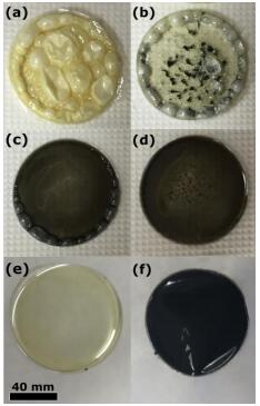 Figure 1. Various issues with solution casting are listed, as well as optical images of the outcomes of these manufacturing issues: (a) high volume-to-surface-area ratio, (b) poor dispersion of the MWCNT as well as a marginally high volume-to-surface-area ratio, (c) slanted drying surface resulting in a nonhomogeneous thickness throughout final solution-cast substrate, and (d) curved aluminum dish resulting in reagglomeration of MWCNTs near the center of the sample. Examples of ideal solution-casted (e) PPP and (f) a MWCNT-PPP composite are shown for comparison.
Various methods to distribute the MWCNTs into the optimized chloroform-PPP solution were attempted, including mixing by hand, vortexing at 3200 rpm for up to one hour, and shaking at 600 rpm for up to 24 hours. Amongst the methods attempted the most effective was sonication for four minutes. Sonication of the composite solution in durations exceeding the four-minute threshold produced no change in appearance of the final product, while sonication for shorter durations resulted in noticeable agglomerations. Apparent fluid viscosity and mechanical properties of pure PPP solvent-cast materials not containing nanotubes were analyzed and showed no change from standard mixing described in the previous section, indicating that the sonication process didn't affect the material properties of the PPP. Pulsing of the sonication was utilized to limit heating of the solution. Thermocouple measurement showed that under constant sonication the temperature of the solution increased more than 28 ℃ above room temperature, whereas pulsing resulted in a max temperature increase of 9 ℃ from room temperature over a four-minute test duration.
Chloroform solvent-cast materials after solvent evaporation had thicknesses averaging 0.10 ± 0.04 mm. Volume fractions exceeding 7 vol.% MWCNT would occasionally fracture or tear in attempts to remove them due to their thin and brittle nature, rendering the sample useless for future testing. Beyond 10 vol.% this issue was exacerbated, leading to frequent failures of films during removal from the aluminum dish. Furthermore, the higher volume fraction composites resulted in a final composite with a rougher surface due to larger areas of concentrated MWCNT agglomerates.
For adequate material characterization, sample preparation of the composites needed to be well controlled. Several issues noted during solvent-casting as well as examples of successful films can be seen in Figure 1. For instance, limiting the volume to free surface area ratio of the poured solution was key to producing a satisfactory result. If the total volume was too large relative to the amount of free surface in the pour, this would initially result in a thicker film after 48 hours of chloroform evaporation in air, but during further drying under vacuum would result in a bubbled surface as the bulk of the remaining chloroform was removed from of the sample. An extreme example of this is shown in Figure 1a. Finally, solutions needed to be poured into a dish that was both very flat and placed on a flat surface, otherwise films of variable thickness and MWCNT dispersion would result. Several side effects of a curved or slanted aluminum dish during the evaporative solidification process can be seen in Figure 1b–d. In Figure 1e, f, these show examples of successfully solvent-cast PPP and a MWCNT-PPP composite, respectively. Overwhelmingly, the issues seen in the casting process arose in areas where the distance to the free surface was too high for effective mass transport of the chloroform. For example, if the bottom of the aluminum casting dish was convex, the PPP-chloroform solution would pool around the edges of the dish, which would create a high localized thickness and, if a composite material was being produced, re-agglomeration of the MWCNT would also occur.
An additional variable that required careful control was the chloroform evaporation rate. If the chloroform was allowed to evaporate in an uncontrolled environment, the rate was too fast, resulting in re-agglomeration of the MWCNTs in the solution. Therefore, during initial solvent evaporation, covering the dish tightly served to control this evaporation rate by transforming the relative partial pressure of the chloroform in the air space, and thus the diffusion rate across the free surface boundary. To ensure any remaining chloroform in the material was removed, cast films were soaked in methanol to aid in the removal of any excess chloroform still trapped in the film.
Bright-field transmission electron micrographs of the MWCNTs used in this study are seen in Figure 2. The average and standard deviation of tube diameters was measured to be 16.5 ± 9 nm, with a maximum size of 34 nm and a minimum of 6.5 nm, as determined from ten representative TEM micrographs. The lengths of the MWCNT are orders of magnitude larger than these diameters, and are not quantified. However, the lengths are stated by the manufacturer to be between 0.5 and 2 µm, which seemed a reasonable value from results observed in subsequent SEM imaging. Catalysts from the chemical vapor deposition manufacturing were also found distributed with the sample of tubes, visible as darker contrast spheres in the TEM images [44]. A sample of multiple tubes can be seen in Figure 2a, while a section of a single tube at higher magnification is seen in Figure 2b. At this magnification, the individual concentric walls of the multiwall tube can be deciphered. Though it is expected to be present, the –COOH functionalization of the tubes is undetectable through this technique.
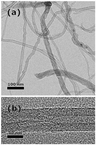 Figure 2. Bright-field TEM micrographs of the MWCNTs showing (a) multiple MWCNTs of varying diameters with some interspersed catalyst and (b) higher magnification on a single multiwall tube, showing the multiple shell nature of the tubes. Overall tube lengths were indeterminate at these magnifications because of limited field of view.
SEM micrographs in Figure 3 are of an edge-on view of a fractured cross-section from a 10 vol.% MWCNT in the PPP matrix. The sample was observed at lower magnifications, highlighting the relative distribution and character of the MWCNTs in the PPP matrix, seen in Figure 3a, and at higher magnifications to highlight how individual MWCNTs interacted first with each other and second the PPP matrix material. The inset area highlighted in white on Figure 3a, is shown in Figure 3b, while the area highlighted in black is shown in Figure 3c. The micrographs are compilations of both BSD and semi-transparent I-L images overlaid on top of each other. In this case, the BSD aids in depth perception while the I-L accentuates the MWCNTs themselves, appearing as individual spots with high brightness in contrast to their surroundings. The relative distribution of the MWCNTs in the matrix can be seen in Figure 3a, where both large MWCNT agglomerations, on the order of tens of micrometers, can be seen intermixed with more homogeneous areas of PPP and MWCNT spread throughout the material.
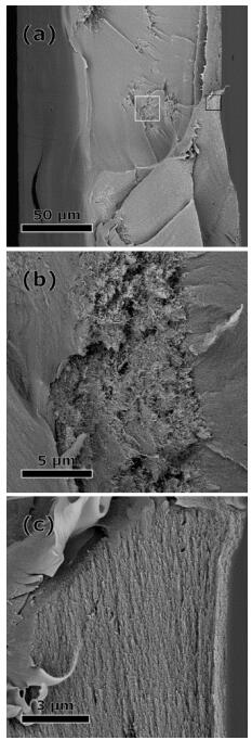 Figure 3. Edge-on composite SEM micrographs of the fracture surface of a 10 vol.% sample. Images are comprised of overlaid in-lens and backscatter electron detector data. Backscatter aids in depth perception, while in-lens highlights individual MWCNT's within the matrix. (a) Micrograph of the full thickness of the sample with the free surface during casting located on the left of the image. Insets highlighted for detail (a) are represented in (b) from the white box, showing an agglomeration area, and (c) from the black box, showing an area of higher homogenization.
It appears that these agglomerations acted as possible locations for crack nucleation and growth in the bending fracture that occurred on the observed sample, with hackle regions apparently emanating from the agglomeration. This can be seen in the large agglomeration on the left side of the sample near the top of the image in Figure 3a. Closer observation of an agglomeration region can be seen in Figure 3b. At this scale, individual MWCNTs are clearly visible. In the central part of the agglomeration, there appears to be a higher ratio of MWCNTs, with a lower dispersion of the PPP, though the PPP is still observable somewhat within. In addition, in these regions the nanotubes appear to have a much higher degree of random orientation. Moving away from the center of the agglomeration to an adjacent area however produces a more uniform distribution of MWCNTs with the PPP. As such, on close inspection, individual nanotubes can be seen jutting out of the fracture surface, clearly within the PPP matrix.
On further inspection of Figure 3a, this distribution of MWCNTs protruding from the PPP can be noted throughout the thickness of the sample save for areas of clear agglomerations where the MWCNTS seem more energetically favorable to bond with each other instead of the matrix. These agglomerations are visible again as individual spots with higher relative brightness. However, although MWCNTs are seen to be present across the entire cross section, it is also apparent that there is some spatial distribution gradient increasing when moving from the left edge to the right edge. In this case, the left edge would have been the free surface during the solvent-casting process. An emphasis of this area can be seen in Figure 3c. Here we see MWCNTs aligning with the sample edge, visible in the bottom right quadrant of the inset. This region highlights a strong interface of the MWCNTs and the PPP matrix, though there is one area devoid of MWCNTs. It is here that the PPP appears to have underwent a crazing deformation process during fracturing of the sample for imaging.
The elastic modulus of the solvent-cast PPP calculated from tensile testing was determined to be E = 4.2 ± 0.2 GPa by curve fitting a line within the elastic region of the deformation process, and on average tested samples would fracture at just over a strain to failure of ԑf = 13 ± 2.3% with an ultimate tensile strength of 96 ± 5.1 MPa. Using this data as a baseline, the effect of the MWCNT reinforcement on the mechanical properties was analyzed. The stress-strain behavior of the solvent-cast PPP was compared against a selection of PPP-MWCNT composites (Figure 4), while the highlights from the tensile properties were measured and compared as a function of MWCNT concentration (Figure 5). Like the bulk PPP, stress-strain behavior of the composites manufactured with volume fractions between 1 and 6 vol.% show yielding behavior prior to failure. With as little as the addition of 1 vol.% of reinforcement to the PPP, the strain-to-failure drops from an average of 13% to 5%. Throughout the range of composites, the modulus of elasticity does not appear to be significantly affected, with the modulus measurements within the standard deviation of the polymer matrix for all materials. There was, however, a change in the ultimate tensile stress, σUTS, where values ranged from a minimum of 98 MPa to maximum of 121 MPa. Throughout this analysis, it was noted that ultimate failure strength and elongation to failure were relatively repeatable with little variation between self-similar measurements. This is demonstrated the standard deviation as displayed by the error bars in Figure 5.
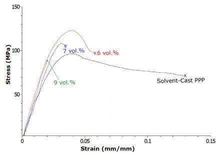 Figure 4. Plot of characteristic stress-strain behavior for select volume fractions of small functionalized composites in comparison to 6 vol.%, 7 vol.%, and 9 vol.% are shown in comparison with the solution casted PPP. The volume fraction of 6 vol.% represents the maximum realized benefits of MWCNT reinforcement, 7 vol.% displays the stark drop-off of mechanical properties measured, and 9 vol.% further highlights the drop-off of mechanical properties.
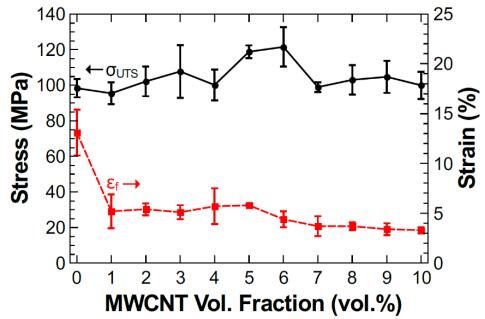 Figure 5. Ultimate tensile strength (σUTS) and strain to failure (εf) plotted within one standard deviation as a function of volume fraction MWCNT in the MWCNT-PPP composites.
Increasing MWCNT volume fraction beyond 10 vol.% resulted in exceedingly brittle materials which would fracture upon removal of the aluminum dish or in the punch process; therefore, volume fractions beyond this limit were not tested mechanically. Beyond the 6 vol.% mark, there is a transition in the characteristic stress-strain behavior from ductile to brittle as composites fail prior to yielding. Unexpected fracture was also noted in the removal of the films from the aluminum dish at volume fractions above 6%. Above this volume fraction removing in-tact films was cumbersome, with many samples tearing or breaking upon removal.
The conductivity of PPP-MWCNT composites was investigated by measuring resistivity and normalizing it to the sample dimensions (Figure 6). Overall, the conductivity of the composites approaches a plateau on the log scale beginning at 5 vol.% and continuing to 20 vol.%. Over this plateau, the conductivity increases about 300% from 3.5 × 10⁻⁴ S/cm ± 9.8 × 10⁻⁷ S/cm to 1.02 × 10⁻³ S/cm ± 5.2 × 10⁻⁵ S/cm. However, this increase is minor when compared with the 2 orders of magnitude jump in resistivity seen over a transition from 3 to 5 vol.%, where conductivity is first measured at 4.5 × 10⁻⁶ S/cm ± 2.1 × 10⁻⁷ S/cm at 3 vol.%. When composites were manufactured using lower volume fractions of material than 3 vol.%, no measurable conductivity was recorded.
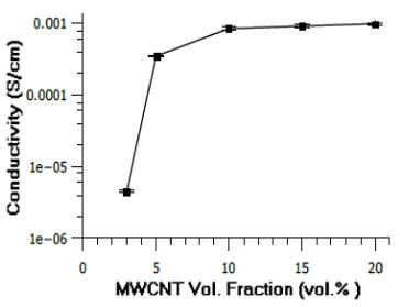 Figure 6. Comparisons of conductivity of the MWCNT-PPP composites shown within one standard deviation on a logarithmic scale. Conductivity was measured at 1, 2, 3, 4, 5, 10, 15, and 20 volume%. Volume fractions of 1% and 2% showed no measurable resistance values. Conductivity is normalized by sample dimensions.
As the evaporation rate of chloroform was so rapid, if the chloroform-PPP solution was left fully exposed to air a solid layer of PPP would form on the top of the solution. This effectively trapped the residual solution which would not allow for diffusion of the chloroform out of the solution. To mitigate this issue, the aluminum dish used for evaporation was covered tightly with aluminum foil. This effectively transformed the relative partial pressure of the chloroform between the free surface of the solution and the air trapped between the dish and the cover. Thus, the diffusion rate across the free surface boundary was controlled and evaporation occurred at a lower rate not allowing the PPP to solidify on the surface and removing nearly all the chloroform from the PPP.
Issues of large volume-to-surface-area ratios in chloroform-PPP films where large bubbles appear on the surface are exhibited in Figure 1a. As these bubbles render the films useless, manufacturing thicker films was limited using the exact methods outlined here and is likely caused by a similar diffusion limitation. As the outer layers of the polymer become solid and complete evaporation of solvent cannot be achieved. The outcome of these samples is strikingly similar to films using dichloromethane as a solvent despite any increase in volume of the samples. These current limitations should also be of note for future applications. Processing the material though solvent-casting has some outstanding potential to make composite materials of this form more appealing. Unfortunately, although the final material thickness would be ideal for a thin film or coating, and current limitations on the thickness noted in this study may be elevated with more advanced techniques, this remains beyond the scope of this study.
During initial studies, PPP was solvent-cast as described in the Section 2, with the exception of soaking the materials in methanol for 24 hours. Preliminary mechanical characterization revealed properties much lower than expected from the literature, with an average elastic modulus of 2.8 ± 0.4 GPa and an average strain-to-failure of ԑf = 7.2 ± 3.1%, values which were nearly half of what was anticipated [7]. It was determined that the discrepancy between solvent-cast PPP and previously studied materials is likely due to the interaction between the chloroform and the PPP powder or due to some effects of residual solvent retained in the material after drying. To remove excess chloroform from the final solvent-cast materials, samples for characterization were soaked in methanol for 24 hours. Several studies have investigated soaking polymers and polymer films in methanol to reduce the amount of solvent swelled in the films [45,46,47]. As the mechanical properties were positively impacted by the soaking in methanol, it suggests that excess chloroform trapped in the PPP and PPP composite materials can play a large role in diminishing the mechanical properties. However, as the values of the solvent-casted films, 4.2 GPa modulus of elasticity and 96 MPa σUTS, still do not reach lower boundary values seen in previous studies of PrimoSpire PR-250 (5 GPa and 140 MPa modulus and σUTS, respectively) [4,7]. This indicates that there may still be some remaining chloroform in the sample which cannot be removed through this process, or that the chloroform is being replaced to some extent by the methanol, which also has some negative effects on mechanical properties. While these effects persist, measured values after soaking in methanol are much closer to target values than those affected by the excess chloroform with modulus values of 2.8 GPa.
During the manufacturing process of the composite films, the high-energy process of sonication heats up the material as it is perturbed. Pulse sonication was utilized to avoid any unwanted effects of heat during manufacturing, the total introduction of energy from the sonication. If temperatures from sonication became too great, the PPP-chloroform mixture would often begin to boil, which indicates that temperatures likely approached 61 ℃, the boiling point of chloroform. Neglecting any additional effect of heating, boiling of the chloroform leads to an increased ratio of PPP to chloroform, which increases the viscosity of the mixture leading to the associated manufacturing issues of the solvent-casting. As the mechanical properties of the PPP were not affected by the sonication process, this mixing method does not appear to have any drawbacks and yields improved nanotube dispersion. Previous studies have observed increased influences on properties when dispersing MWCNTs using tip sonication, therefore it was chosen as the preferred method for this study [14].
TEM results of the CNTs suggest that the carbon nanotubes provided for this experiment are multi-walled in nature and manufacturers dimension specifications reflect what is seen. From the TEM results seen in Figure 2, it is clear the manufacturing process used for these tubes is via a vapor deposition method as determined by the observations of the resultant catalyst remaining in the system. However, there is little reason to believe that this remaining catalyst should have any impact on the behavior of the composite material. Though there is no way of directly observing the –COOH bonds using the conventional TEM methods used here, there is reason to believe that this functionalization will have a large impact on the effectiveness of the MWCNT, by creating a larger affinity for the PPP than non-functionalized MWCNT would, ultimately assisting in decreasing the agglomeration size.
Though the agglomerations were limited in size, as functionalized MWCNT were used and as the processing methods mitigated re-agglomeration in the solvent, bundles of MWCNTs were not completely eradicated. Such agglomerating structures are common in composites manufactured with MWCNT reinforcement [14,48,49,50,51,52,53,54], and careful preparation is required to minimize their size and distribute them homogenously throughout. That being said, a well-mixed solution is necessary for the manufacturing of a strong and functional composite material. One way to mitigate agglomerations and increase homogeneity is, first and foremost, by using a solvent-cast technique; some of the agglomeration issues can be immediately alleviated through this technique when compared with, for example, a more typical powder press method. As the PPP-MWCNT mixture is entirely suspended in the solvent, MWCNT dispersion is simplified by the variety of mixing methods that become available for use. This includes multiple sonication techniques, one of which is tip-sonication which produced the best results in this study.
Results from the final method utilized here can be seen in the SEM images, shown in Figure 3. At 10 vol.% MWCNT, some agglomerated MWCNT pockets are seen through the thickness of the sample with an apparently homogenous mixture of MWCNT and PPP everywhere else. In composites consisting of large volume fractions of MWCNTs these agglomerations become more common. This is noted even in traditionally manufactured high temperature thermoplastic-CNT composites. Ribeiro et al. reports that in MWCNT-PPS composite, agglomerations are more prevalent in 4 wt% reinforced composite as opposed to 1 wt% composite [11]. Even though great strides were made in minimizing the agglomerations via the method developed here, the agglomerations that are present appear to act as nucleation sites for crack propagation shown by the hackle region emanating from the larger agglomerations in the SEM image. This partially explains the increasing brittle nature with an increase in MWCNT composition shown in the mechanical testing. As the MWCNT composition increases so does the likelihood of agglomerations, both in number and in size. These locations, without any PPP matrix, can no longer effectively transfer the load, and instead act as stress-concentrating internal voids. There is also some variability in distribution of these agglomerations through the thickness of the observed sample. As indicated, the free surface of the sample would have been on the left side of the SEM images and includes the side with more agglomerations. The increase in density of agglomerations near the free surface is likely due to two effects. The first effect is the possibility of a re-agglomeration process occurring as the chloroform moved towards the free surface; the second effect is the lower density of the agglomerations within the homogeneous mixture tended to migrate to the free surface during the solidification process.
At low-volume fractions of MWCNT, up to 6 vol.%, the PPP composite's mechanical properties increase as expected with composite theory when compared with the baseline solvent-cast PPP. With an increase in reinforcement, the strain-to-failure of the composite materials decreases significantly, while the strength increases as seen in Figures 4 and 5. However, as the concentration increases past low-volume fractions the strength actually begins to decrease. Therefore, not only does the MWCNT reinforcement act to increase the strength of the composites when well distributed, but due to the agglomerations, also induces a defect in the material which influences the ductility of the composites. Despite increasing amounts of added reinforcement, the benefits of MWCNTs are not fully realized, only causing minor changes in the ultimate strength and keeping the modulus relatively constant across the range of volume fraction tested. While theoretical, the addition of the MWCNT should increase the stiffness and strength of these materials according to composites theory, but there is competition of other factors such as adhesion of the MWCNT to the PPP matrix or clustering of the reinforcement into agglomerations. In the 5 vol.% and 6 vol.% composites, an optimal concentration of MWCNTs is reached in the current study such that it leads to an increase in ultimate tensile strength, with the matrix adequately transferring the load to the reinforcement while overcoming the issues that cause detrimental effects with further increase in MWCNT concentration.
As the volume fraction of MWCNTs increases, pockets of agglomerations become larger and more numerous, enough to dictate and cause premature failure. It is expected that without the competing negative effects, the strength of the composites would show an increasing trend in ultimate tensile strength as shown in many other nano-reinforced composite materials [55,56,57,58]. The drop in mechanical properties is consistent with the premature failure 7 vol.% threshold, where sample removal would lead to tearing of the films. It is expected this tearing occurred when films are deformed to strains that would otherwise be in the elastic regime. It is also expected that the MWCNT gradient noted in SEM played a role in diminishing the mechanical properties of the final composites as the tested films trended further from a homogenous nature.
The asymptotic behavior of the conductivity of MWCNTs composites is as expected as it has been noted in previous studies [51]. The conductivity of low-volume fraction materials (1 vol.% and 2 vol.%) is unmeasurably low; despite this, it is likely that the material is still conductive to a very small degree. Conductivity values on the order of magnitude of 10−3 S/cm as observed for higher volume fractions in Figure 6 are well within expected values when compared with previous studies [11,14,51,59]. While values of conductivity are not as large as some MWCNT-polymer composites [14]—despite the fact that PPP alone is a relatively strong electrical insulator [60] when compared with other polymers—the likely cause of this drop in conductivity is due to the surface modifcations of the MWCNTs [61,62]. It is unlikely that increasing volume fractions of MWCNT beyond the concentrations investigated in this study would further increase the conductivity. Throughout the range of MWCNT reinforcements tested the materials reached the percolation threshold at approximately 5 vol.% reinforcement, maximizing electrical conductivity of the samples.
A thin film of PPP thermoplastic was fabricated via a novel solvent-casting method, opening the door to many potential new applications for this strong polymer. Employing the solvent-casting methods developed here could realize potential PPP films suitable for creation of thin substrates or as coatings to harness the material's superior scratch resistant or biocompatible properties. Solvent-casting of PPP allows for mitigation of the high manufacturing temperatures and pressures traditionally required for PPP, and could be applied as a coating to materials which have previously been difficult or impossible to coat. The mechanical properties of the resulting polymer film were experimentally measured, marking the first time solvent-cast PPP has been characterized. The solvent-casted PPP shows an average modulus of 4.2 GPa, an average ultimate tensile strength of 96 MPa, and an average strain-to-failure of 13%.
Furthermore, manufacturing composite materials via solvent-casting was investigated using functionalized MWCNTs. Properties of the solvent-cast composites were investigated as a function of increasing volume fraction of MWCNT within a PPP matrix, and their mechanical and electrical properties were measured. Overall, solvent-casting proved to be an effective manufacturing method for not just PPP substrates, but MWCNT-PPP composites as well. However, despite using sonication to disperse the MWCNT in the polymer matrix, some agglomerations were still observed using microscopy techniques and are expected to hinder the optimal strength the material could reach. The influence of the MWCNT on the mechanical properties of solvent-cast composites was relatively little, with the exception of a drop-off in strain-to-failure, with ultimate tensile strength increasing to 121 MPa and elastic modulus remaining relatively constant with increasing volume fraction of reinforcement. It is expected that this can be improved with further studies in processing to further remove the agglomerated species of MWCNT and reduce re-agglomeration while suspended in solution during the solidification process. The electrical conductivity of the measured composites reached near maximum potential around 5 percent volume fraction, with little change noted with further increases in carbon nanotube density of the composites. The maximum conductivity observed was 1.02 × 10⁻³ S/cm. At present, solvent-cast thin film PPP and composites can be easily manufactured, although further investigations are necessary to allow for increased material thicknesses of cast PPP and improvements upon the mechanical characteristics of the composites.
The authors would like to acknowledge the Leibniz Universit t Hannover; especially Anja Krabbenhöft and Dr. Hans Maier for their aid in scanning electron microscopy. MWCNTs and PPP graciously provided by Haydale LLC and Solvay Specialty Polymers LLC, respectively. Special thanks to the University of Wyoming School of Energy Resources for financial support.
There is no conflict of interest regarding the publication of this manuscript.
| [1] |
Nunes JP, Silva JF, Velosa JC, et al. (2009) New thermoplastic matrix composites for demanding applications. Plast Rubber Compos 38: 167–172. doi: 10.1179/174328909X387946

|
| [2] | Dean D, Husband M, Trimmer M (1998) Time–temperature-dependent behavior of a substituted poly(paraphenylene): Tensile, creep, and dynamic mechanical properties in the glassy state. J Polym Sci Pol Phys 36: 2971–2979. |
| [3] |
Friedrich K, Burkhart T, Almajid AA, et al. (2010) Poly-Para-Phenylene-Copolymer (PPP): A High-Strength Polymer with Interesting Mechanical and Tribological Properties. Int J Polym Mater Po 59: 680–692. doi: 10.1080/00914037.2010.483211
|
| [4] |
Frick CP, DiRienzo AL, Hoyt AJ, et al. (2014) High-strength poly(para-phenylene) as an orthopedic biomaterial. J Biomed Mater Res A 102: 3122–3129. doi: 10.1002/jbm.a.34982
|
| [5] |
Hoyt AJ, Yakacki CM, Fertig III RS, et al. (2015) Monotonic and cyclic loading behavior of porous scaffolds made from poly(para-phenylene) for orthopedic applications. J Mech Behav Biomed 41: 136–148. doi: 10.1016/j.jmbbm.2014.10.004
|
| [6] |
DiRienzo AL, Yakacki CM, Frensemeier M, et al. (2014) Porous poly(para-phenylene) scaffolds for load-bearing orthopedic applications. J Mech Behav Biomed 30: 347–357. doi: 10.1016/j.jmbbm.2013.10.012
|
| [7] | Collins DA, Yakacki CM, Lightbody D, et al. (2016) Shape-memory behavior of high-strength amorphous thermoplastic poly(para-phenylene). J Appl Polym Sci 133: 1–10. |
| [8] |
Almajid A, Friedrich K, Noll A, et al. (2013) Poly-para-phenylene-copolymers (PPP) for extrusion and injection moulding Part 1——molecular and rheological differences. Plast Rubber Compos 42: 123–128. doi: 10.1179/1743289812Y.0000000045
|
| [9] | Pei X, Friedrich K (2012) Sliding wear properties of PEEK, PBI and PPP. Wear 274–275: 452–455. |
| [10] |
Ma Y, Cong P, Chen H, et al. (2015) Mechanical and Tribological Properties of Self-Reinforced Polyphenylene Sulfide Composites. J Macromol Sci B 54: 1169–1182. doi: 10.1080/00222348.2015.1061845
|
| [11] |
Ribeiro B, Pipes RB, Costa ML, et al. (2017) Electrical and rheological percolation behavior of multiwalled carbon nanotube-reinforced poly(phenylene sulfide) composites. J Compos Mater 51: 199–208. doi: 10.1177/0021998316644848
|
| [12] |
Mahat KB, Alarifi I, Alharbi A, et al. (2016) Effects of UV Light on Mechanical Properties of Carbon Fiber Reinforced PPS Thermoplastic Composites. Macromol Symp 365: 157–168. doi: 10.1002/masy.201650015
|
| [13] |
Kuo MC, Huang JC, Chen M, et al. (2003) Fabrication of High Performance Magnesium/Carbon-Fiber/PEEK Laminated Composites. Mater Trans 44: 1613–1619. doi: 10.2320/matertrans.44.1613
|
| [14] |
Martin AC, Lakhera N, DiRienzo AL, et al. (2013) Amorphous-to-crystalline transition of Polyetheretherketone-carbon nanotube composites via resistive heating. Compos Sci Technol 89: 110–119. doi: 10.1016/j.compscitech.2013.09.012
|
| [15] |
Garcia-Gonzalez D, Rusinek A, Jankowiak T, et al. (2015) Mechanical impact behavior of polyether-ether-ketone (PEEK). Compos Struct 124: 88–99. doi: 10.1016/j.compstruct.2014.12.061
|
| [16] |
Bishop MT, Karasz FE, Russo PS, et al. (1985) Solubility and Properties of a Poly(aryl ether ketone) in Strong Acids. Macromolecules 18: 86–93. doi: 10.1021/ma00143a014
|
| [17] | Shukla D, Negi YS, Kumar V (2013) Modification of Poly(ether ether ketone) Polymer for Fuel Cell Application. J Appl Chem 2013. |
| [18] |
Wang X, Li Z, Zhang M, et al. (2017) Preparation of a polyphenylene sulfide membrane from a ternary polymer/solvent/non-solvent system by thermally induced phase separation. RSC Adv 7: 10503–10516. doi: 10.1039/C6RA28762J
|
| [19] |
Natori I, Natori S, Sekikawa H, et al. (2008) Synthesis of soluble poly(para-phenylene) with a long polymer chain: Characteristics of regioregular poly(1,4-phenylene). J Polym Sci Pol Chem 46: 5223–5231. doi: 10.1002/pola.22851
|
| [20] |
Marvel CS, Hartzell GE (1959) Preparation and Aromatization of Poly-1,3-cyclohexadiene1. J Am Chem Soc 81: 448–452. doi: 10.1021/ja01511a047
|
| [21] | Cochet M, Maser WK, Benito AM, et al. (2001) Synthesis of a new polyaniline/nanotube composite: "in-situ" polymerisation and charge transfer through site-selective interaction. Chem Commun 1450–1451. |
| [22] |
Olifirov LK, Kaloshkin SD, Zhang D (2017) Study of thermal conductivity and stress-strain compression behavior of epoxy composites highly filled with Al and Al/f-MWCNT obtained by high-energy ball milling. Compos Part A-Appl S 101: 344–352. doi: 10.1016/j.compositesa.2017.06.027
|
| [23] |
Overney G, Zhong W, Tomanek D (1993) Structural rigidity and low frequency vibrational modes of long carbon tubules. Z Phys D-Atoms, Molecules and Clusters 27: 93–96. doi: 10.1007/BF01436769
|
| [24] |
Spitalsky Z, Tasis D, Papagelis K, et al. (2010) Carbon nanotube-polymer composites: Chemistry, processing, mechanical and electrical properties. Prog Polym Sci 35: 357–401. doi: 10.1016/j.progpolymsci.2009.09.003
|
| [25] | Khare R, Bose S (2005) Carbon Nanotube Based Composites——A Review. J Min Mater Charact Eng 4: 31–46. |
| [26] |
Schadler LS, Giannaris SC, Ajayan PM (1998) Load transfer in carbon nanotube epoxy composites. Appl Phys Lett 73: 3842–3844. doi: 10.1063/1.122911
|
| [27] |
Frankland SJV, Caglar A, Brenner DW, et al. (2002) Molecular simulation of the influence of chemical cross-links on the shear strength of carbon nanotube-polymer interfaces. J Phys Chem B 106: 3046–3048. doi: 10.1021/jp015591+
|
| [28] |
Tsuda T, Ogasawara T, Deng F, et al. (2011) Direct measurements of interfacial shear strength of multi-walled carbon nanotube/PEEK composite using a nano-pullout method. Compos Sci Technol 71: 1295–1300. doi: 10.1016/j.compscitech.2011.04.014
|
| [29] |
Calvert P (1999) Nanotube Composites: A recipe for strength. Nature 399: 210–211. doi: 10.1038/20326
|
| [30] |
Tasis D, Tagmatarchis N, Bianco A, et al. (2006) Chemistry of carbon nanotubes. Chem Rev 106: 1105–1136. doi: 10.1021/cr050569o
|
| [31] |
Ma PC, Siddiqui NA, Marom G, et al. (2010) Dispersion and functionalization of carbon nanotubes for polymer-based nanocomposites: A review. Compos Part A-Appl S 41: 1345–1367. doi: 10.1016/j.compositesa.2010.07.003
|
| [32] |
Grady BP (2010) Recent developments concerning the dispersion of carbon nanotubes in polymers. Macromol Rapid Comm 31: 247–257. doi: 10.1002/marc.200900514
|
| [33] |
Jyoti J, Babal AS, Sharma S, et al. (2018) Significant improvement in static and dynamic mechanical properties of graphene oxide-carbon nanotube acrylonitrile butadiene styrene hybrid composites. J Mater Sci 53: 2520–2536. doi: 10.1007/s10853-017-1592-6
|
| [34] |
Song YS, Youn JR (2005) Influence of dispersion states of carbon nanotubes on physical properties of epoxy nanocomposites. Carbon 43: 1378–1385. doi: 10.1016/j.carbon.2005.01.007
|
| [35] |
Shi DL, Feng XQ, Huang YY, et al. (2004) The effect of nanotube waviness and agglomeration on the elastic property of carbon nanotube-reinforced composites. J Eng Mater-T ASME 126: 250–257. doi: 10.1115/1.1751182
|
| [36] |
Fiedler B, Gojny FH, Wichmann MHG, et al. (2006) Fundamental aspects of nano-reinforced composites. Compos Sci Technol 66: 3115–3125. doi: 10.1016/j.compscitech.2005.01.014
|
| [37] |
Strano MS, Dyke CA, Usrey ML, et al. (2003) Electronic structure control of single-walled carbon nanotube functionalization. Science 301: 1519–1522. doi: 10.1126/science.1087691
|
| [38] |
Banerjee S, Kahn MGC, Wong SS (2003) Rational chemical strategies for carbon nanotube functionalization. Chem-Eur J 9: 1898–1908. doi: 10.1002/chem.200204618
|
| [39] |
Yang K, Gu M, Guo Y, et al. (2009) Effects of carbon nanotube functionalization on the mechanical and thermal properties of epoxy composites. Carbon 47: 1723–1737. doi: 10.1016/j.carbon.2009.02.029
|
| [40] |
Sahoo NG, Rana S, Cho JW, et al. (2010) Polymer nanocomposites based on functionalized carbon nanotubes. Prog Polym Sci 35: 837–867. doi: 10.1016/j.progpolymsci.2010.03.002
|
| [41] |
Silva JF, Nunes JP, Velosa JC, et al. (2010) Thermoplastic matrix towpreg production. Adv Polym Tech 29: 80–85. doi: 10.1002/adv.20174
|
| [42] | Vuorinen A (2010) Rigid Rod Polymers Fillers in Acrylic Denture and Dental Adhesive Resin Systems. |
| [43] |
Kwok N, Hahn HT (2007) Resistance heating for self-healing composites. J Compos Mater 41: 1635–1654. doi: 10.1177/0021998306069876
|
| [44] |
Delzeit L, Nguyen CV, Chen B, et al. (2002) Multiwalled carbon nanotubes by chemical vapor deposition using multilayered metal catalysts. J Phys Chem B 106: 5629–5635. doi: 10.1021/jp0203898
|
| [45] | Caneba G (2010) Product Materials, In: Free-radical retrograde-precipitation polymerization (FRRPP): novel concept, processes, materials, and energy aspects, Springer Science & Business Media, 199–252. |
| [46] | Xu Z, Wan L, Huang X (2009) Surface Modification by Graft Polymerization, In: Surface Engineering of Polymer Membranes. Advanced Topics in Science and Technology in China, Springer, Berlin, Heidelberg, 80–149. |
| [47] |
Kubo T, Im J, Wang X, et al. (2014) Solvent induced nanostructure formation in polymer thin films: The impact of oxidation and solvent. Colloid Surface A 444: 217–225. doi: 10.1016/j.colsurfa.2013.12.052
|
| [48] |
Ajayan PM, Stephan O, Colliex C, et al. (1994) Aligned carbon nanotube arrays formed by cutting a polymer resin-nanotube composite. Science 265: 1212–1214. doi: 10.1126/science.265.5176.1212
|
| [49] |
Haggenmueller R, Gommans HH, Rinzler AG, et al. (2000) Aligned single-wall carbon nanotubes in composites by melt processing methods. Chem Phys Lett 330: 219–225. doi: 10.1016/S0009-2614(00)01013-7
|
| [50] |
Puglia D, Valentini L, Kenny JM (2003) Analysis of the cure reaction of carbon nanotubes/epoxy resin composites through thermal analysis and Raman spectroscopy. J Appl Polym Sci 88: 452–458. doi: 10.1002/app.11745
|
| [51] |
Park C, Ounaies Z, Watson KA, et al. (2002) Dispersion of single wall carbon nanotubes by in situ polymerization under sonication. Chem Phys Lett 364: 303–308. doi: 10.1016/S0009-2614(02)01326-X
|
| [52] |
Qian D, Dickey EC, Andrews R, et al. (2000) Load transfer and deformation mechanisms in carbon nanotube-polystyrene composites. Appl Phys Lett 76: 2868–2870. doi: 10.1063/1.126500
|
| [53] |
Allaoui A, Bai S, Cheng HM, et al. (2002) Mechanical and electrical properties of a MWNT/epoxy composite. Compos Sci Technol 62: 1993–1998. doi: 10.1016/S0266-3538(02)00129-X
|
| [54] |
Ajayan PM, Schadler LS, Giannaris C, et al. (2000) Single-walled carbon nanotube–polymer composites: strength and weakness. Adv Mater 12: 750–753. doi: 10.1002/(SICI)1521-4095(200005)12:10<750::AID-ADMA750>3.0.CO;2-6
|
| [55] |
Li Y, Zhang H, Porwal H, et al. (2017) Mechanical, electrical and thermal properties of in-situ exfoliated graphene/epoxy nanocomposites. Compos Part A-Appl S 95: 229–236. doi: 10.1016/j.compositesa.2017.01.007
|
| [56] |
Zhang Y, Park SJ (2017) Enhanced interfacial interaction by grafting carboxylated-macromolecular chains on nanodiamond surfaces for epoxy-based thermosets. J Polym Sci Pol Phys 55: 1890–1898. doi: 10.1002/polb.24522
|
| [57] |
Zhang Y, Rhee KY, Park SJ (2017) Nanodiamond nanocluster-decorated graphene oxide/epoxy nanocomposites with enhanced mechanical behavior and thermal stability. Compos Part B-Eng 114: 111–120. doi: 10.1016/j.compositesb.2017.01.051
|
| [58] |
Sharmila TKB, Antony JV, Jayakrishnan MP, et al. (2016) Mechanical, thermal and dielectric properties of hybrid composites of epoxy and reduced graphene oxide/iron oxide. Mater Design 90: 66–75. doi: 10.1016/j.matdes.2015.10.055
|
| [59] |
Shaffer MSP, Windle AH (1999) Fabrication and characterization of carbon nanotube/poly(vinyl alcohol) composites. Adv Mater 11: 937–941. doi: 10.1002/(SICI)1521-4095(199908)11:11<937::AID-ADMA937>3.0.CO;2-9
|
| [60] |
Rizzatti MR, De Araujo MA, Livi RP (1995) Bulk and surface modifications of insulating poly(paraphenylene sulphide) films by ion bombardment. Surf Coat Tech 70: 197–202. doi: 10.1016/0257-8972(94)02275-U
|
| [61] |
Liu Y, Gao L (2005) A study of the electrical properties of carbon nanotube-NiFe2O4 composites: Effect of the surface treatment of the carbon nanotubes. Carbon 43: 47–52. doi: 10.1016/j.carbon.2004.08.019
|
| [62] |
Park OK, Jeevananda T, Kim NH, et al. (2009) Effects of surface modification on the dispersion and electrical conductivity of carbon nanotube/polyaniline composites. Scripta Mater 60: 551–554. doi: 10.1016/j.scriptamat.2008.12.005
|

Stephan A. Brinckmann, Nishant Lakhera, Chris M. Laursen, Christopher Yakacki, Carl P. Frick. Characterization of poly(para-phenylene)-MWCNT solvent-cast composites[J]. AIMS Materials Science, 2018, 5(2): 301-319. doi: 10.3934/matersci.2018.2.301


 DownLoad:


