


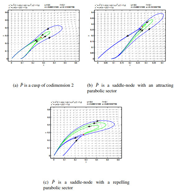
Figure 1.
Phase portraits near $ \bar{P} $.
Citation: Larysa Khomenkova, Mykola Baran, Jedrzej Jedrzejewski, Caroline Bonafos, Vincent Paillard, Yevgen Venger, Isaac Balberg, Nadiia Korsunska. Silicon nanocrystals embedded in oxide films grown by magnetron sputtering[J]. AIMS Materials Science, 2016, 3(2): 538-561. doi: 10.3934/matersci.2016.2.538
| [1] | Mengyun Xing, Mengxin He, Zhong Li . Dynamics of a modified Leslie-Gower predator-prey model with double Allee effects. Mathematical Biosciences and Engineering, 2024, 21(1): 792-831. doi: 10.3934/mbe.2024034 |
| [2] | Manoj K. Singh, Brajesh K. Singh, Poonam, Carlo Cattani . Under nonlinear prey-harvesting, effect of strong Allee effect on the dynamics of a modified Leslie-Gower predator-prey model. Mathematical Biosciences and Engineering, 2023, 20(6): 9625-9644. doi: 10.3934/mbe.2023422 |
| [3] | Hongqiuxue Wu, Zhong Li, Mengxin He . Dynamic analysis of a Leslie-Gower predator-prey model with the fear effect and nonlinear harvesting. Mathematical Biosciences and Engineering, 2023, 20(10): 18592-18629. doi: 10.3934/mbe.2023825 |
| [4] | Saheb Pal, Nikhil Pal, Sudip Samanta, Joydev Chattopadhyay . Fear effect in prey and hunting cooperation among predators in a Leslie-Gower model. Mathematical Biosciences and Engineering, 2019, 16(5): 5146-5179. doi: 10.3934/mbe.2019258 |
| [5] | Rongjie Yu, Hengguo Yu, Chuanjun Dai, Zengling Ma, Qi Wang, Min Zhao . Bifurcation analysis of Leslie-Gower predator-prey system with harvesting and fear effect. Mathematical Biosciences and Engineering, 2023, 20(10): 18267-18300. doi: 10.3934/mbe.2023812 |
| [6] | Kawkab Al Amri, Qamar J. A Khan, David Greenhalgh . Combined impact of fear and Allee effect in predator-prey interaction models on their growth. Mathematical Biosciences and Engineering, 2024, 21(10): 7211-7252. doi: 10.3934/mbe.2024319 |
| [7] | Shuo Yao, Jingen Yang, Sanling Yuan . Bifurcation analysis in a modified Leslie-Gower predator-prey model with fear effect and multiple delays. Mathematical Biosciences and Engineering, 2024, 21(4): 5658-5685. doi: 10.3934/mbe.2024249 |
| [8] | Yuhong Huo, Gourav Mandal, Lakshmi Narayan Guin, Santabrata Chakravarty, Renji Han . Allee effect-driven complexity in a spatiotemporal predator-prey system with fear factor. Mathematical Biosciences and Engineering, 2023, 20(10): 18820-18860. doi: 10.3934/mbe.2023834 |
| [9] | Zhenzhen Shi, Huidong Cheng, Yu Liu, Yanhui Wang . Optimization of an integrated feedback control for a pest management predator-prey model. Mathematical Biosciences and Engineering, 2019, 16(6): 7963-7981. doi: 10.3934/mbe.2019401 |
| [10] | Kunlun Huang, Xintian Jia, Cuiping Li . Analysis of modified Holling-Tanner model with strong Allee effect. Mathematical Biosciences and Engineering, 2023, 20(8): 15524-15543. doi: 10.3934/mbe.2023693 |
Predation is a ubiquitous interaction among species and thus it has been studied extensively. Most predator-prey models are extensions and modifications of the classical Lotka-Volterra model by incorporating many other factors. The obtained theoretical results can guide us to make appropriate policies on ecological protection and ecological sustainable development [1]. One important modification is the Leslie-Gower model described by
|
$ dxdt=rx(1−xK)−P(x)y,dydt=ys(1−ynx), $
|
(1.1) |
where $ x(t) $ and $ y(t) $ stand for the densities of the prey and predator at time $ t $, respectively. Here both species have the logistic growths with respective intrinsic growth rates $ r $ and $ s $ and with the carrying capacities $ K $ for the prey and $ nx $ for the predator (which depends on the density of the prey). $ n $ is a measure of the quality of the prey and $ nx $ is called the Leslie-Gower term [2]. $ P(x) $ is the functional response of predators to prey. Model (1.1) has been extensively studied and promoted (see, for example, [3,4]). Recently, the influence of fear effect and Allee effect on the dynamical behaviors of predator-prey models has attracted many researchers' attention.
Fear effect of predator is a form of indirect predation impacting the prey population [5,6,7]. To some extent, the physiological states of prey are disturbed by the fear effect. As a result, in the long run, the fear effect may lead to a loss in prey population. Meanwhile, the prey suffered from scare usually forage less and then their birth rate decreases which may be not good for the survival of prey's population. There is an example that some birds make anti-predator defenses against the sound of the predator and once perceive danger, they flee from their nests. As far as prey is concerned, frequent exposure to fear and anti-predation behavior will affect their birth rate. Therefore, it is necessary to take into account of fear factor in the predator-prey interaction [8,9,10]. In [11], Wang et al. first modeled the fear effect by introducing a factor $ f(k, y) $, where $ k $ represents the intensity of anti-predator behaviors of the prey caused by fear. See the paper for more detail on the properties of $ f(k, y) $. A recent experiment designed by Elliott et al. [12] demonstrated that Allee effect [13,14,15] can be induced by the fear effect. Moreover, the strong Allee effects [16,17] should be paid more attention, because too large fear intensity will drive the species to extinction.
Allee effect mainly signifies that individual fitness is directly proportionate to population density. Due to the variety of species, the causes of Allee effect are also different. Such as sperm limitation, reproduction facilitation, cooperative breeding, anti-predator behavior and predator satiation. During the last decades, lots have been done for predator-prey models with Allee effects. For example, Merdan [18] investigated the stabilityof a Lotka-Volterra type predator-prey system involving Allee effect; Liu and Dai [19] considered an impulsive predator-prey model with double Allee effects; Wu et al. [20] tried to understand the Allee effect in a commensal symbiosis mode; studied Guan and Chen [21] studied an amensalism model with Allee effect on the second species; and Naik et al. [22] explored the effect of strong Allee effect in a discrete predator-prey model.
On the one hand, based on the experimental observations of Elliott et al. [12], Sasmal [15] proposed and investigated the following predator-prey model with prey subject to Allee effect and fear effect,
|
$ dxdt=rx(1−xK)(x−θ)11+fy−axy,dydt=αaxy−my, $
|
where $ \theta $ and $ f $ are Allee constant and fear factor, respectively. They showed that the cost of fear has no influence on the stability of equilibria. On the other hand, González-Olivares et al. [23] studied the following Leslie-Gower model with Allee effect in prey,
|
$ dxdt=rx(1−xK)(x−m)−qxy,dydt=sy(1−ynx), $
|
where $ m $ represents the Allee effect threshold. Without Allee effect, there is a unique equilibrium, which is globally asymptotically stable. However, with the presence of strong Allee effect, the number of equilibria varies with respect to $ m $. It is shown that the system exhibits local bifurcations including Hopf bifurcation and Bogdanov-Takens bifurcation.
Inspired by these two works [15,23], it is natural and interesting to investigate the combined influence of both Allee effect and fear effect on dynamics of Leslie-Gower predator-prey models. In other words, whether the qualitative structure and bifurcation phenomena will become more complex? The thoretical results will help humans manage ecosystems. Precisely, the model to be studied in this paper is
|
$ dxdt=rx(1−xK)(x−m)11+fy−qxy,dydt=ys(1−ynx), $
|
(1.2) |
where $ r $, $ K $, $ f $, $ q $, $ n $, $ s $, and $ m $ are all positive constants and $ 0 < m < K $. For simplicity of analysis, we introduce new variables
| $ \bar{x} = \frac{x}{K},\quad \bar{y} = \frac{1}{nK}y,\quad \bar{t} = rKt, $ |
and denote
| $ \bar{m} = \frac{m}{K},\quad \bar{q} = \frac{nq}{r},\quad \bar{s} = \frac{s}{rk},\quad \bar{f} = fnK. $ |
Then system (1.2) becomes
|
$ dxdt=x(1−x)(x−m)11+fy−qxy,dydt=ys(1−yx), $
|
(1.3) |
(note that we have dropped the bars here), where $ m $, $ f $, $ q $, and $ s $ are positive constants with $ 0 < m < 1 $.
Though not defined at $ x = 0 $, the dynamical behavior of (1.3) in the absence of prey is of interest. For this end, we take the time scaling $ d t = (1+fy)x d \tau $ to get a new system (still label $ \tau $ as $ t $),
|
$ dxdt=x2(1−x)(x−m)−qx2y(1+fy), $
|
(1.4a) |
|
$ dydt=ys(x−y)(1+fy). $
|
(1.4b) |
This new system with the time scale reaches stable equilibria much faster than the original one. As a result, in the following we only focus on (1.4). Due to the biological background, the initial conditions $ (x(0), y(0))\in\mathbb{R}_+^2 $. Obviously, for such an initial condition, (1.4) has a unique global solution which stays in $ \mathbb{R}_+^2 $.
In the following, we first present the results on boundedness of solutions and the attraction of the origin. Followed is the existence and local stability of equilibria. The results indicate possible occurrence of bifurcations. We thus explore the detail on saddle-node bifurcation of codimension 1, Hopf bifurcation of codimension 1, and Bogdanov-Takens bifurcation of codimension 2. A brief conclusion ends the paper.
We first show the ultimate boundedness of solutions of (1.4).
Proposition 1. Let $ (x(t), y(t)) $ be a solution of (1.4). Then
| $ \limsup\limits_{t\to\infty}x(t)\le 1\quad and\quad \limsup\limits_{t\to\infty}y(t)\le 1. $ |
Proof. We show $ \limsup_{t\to\infty}x(t)\le 1 $ by distinguishing two cases. Firstly, we assume $ x(t)\ge 1 $ for $ t\ge 0 $. Then it follows from (1.4a) that $ x $ is a decreasing function. Denote $ \lim_{t\to\infty}x(t) $ by $ l $. It is easy to see that $ l = 1 $. Next, we assume that $ x(t_0) < 1 $ for some $ t_0\ge 0 $. We claim that, for $ t\ge t_0 $, $ x(t)\le 1 $. Otherwise, there exists a $ t^* > t_0 $ such that $ x(t^*) > 1 $. Let $ x(\hat{t}) = \max\{x(t)\vert t_0\le t\le t^*\} $. As $ \frac{dx(t^*)}{dt} < 0 $, we have $ \hat{t}\in (t_0, t^*) $ and hence $ \frac{dx(\hat{t})}{dt} = 0 $. This is impossible as $ x(\hat{t}) > 1 $, which gives $ \frac{dx(\hat{t})}{dt} < 0 $. The claim is proved. To sum up, $ \limsup_{t\to\infty}x(t)\le 1 $ is proved. Now, for $ \varepsilon_0 > 0 $, there exists $ \breve{t}\ge 0 $ such that $ x(t)\le 1+\varepsilon_0 $ for $ t\ge \breve{t} $. It follows that, for $ t\ge \breve{t} $,
| $ \frac{dy(t)}{dt}\le ys(1+\varepsilon_0-y)(1+fy). $ |
Then arguing similarly as for $ \limsup_{t\to\infty}x(t)\le 1 $, we can get $ \limsup_{t\to\infty}y(t)\le 1+\varepsilon_0 $. As $ \varepsilon_0 $ is arbitrary, we immediately have $ \limsup_{t\to\infty}y(t)\le 1 $.
We start with finding the equilibria to (1.4), which are determined by solutions to
|
$ {x2(1−x)(x−m)−qx2y(1+fy)=0,ys(x−y)(1+fy)=0. $
|
Clearly, (1.4) always admits two positive boundary equilibria $ P_1(m, 0) $ and $ P_2(1, 0) $. Moreover, for a positive equilibrium $ (x, x) $ (or coexistence equilibrium), $ x $ satisfies
|
$ −(1+fq)x2+(m−q+1)x−m=0. $
|
(3.1) |
If $ m-q+1\le 0 $ then (3.1) has no positive roots and hence (1.4) has no positive equilibria. Now assume that $ m-q+1 > 0 $, which implies that $ q < m+1 < 2 $. Denote the discriminant of (3.1) by $ \Delta $ and it can be expressed as a quadratic function of $ m $,
| $ \Delta(m) = m^2-2(2fq+q+1)m+(q-1)^2. $ |
Note that $ \Delta(1) = q(q-4-4f) < 0 $ and $ \Delta(q-1) = 2(1-q)(2+fq) $. It follows that if $ q\ge 1 $ then $ \Delta(m) < 0 $, which again implies that (1.4) has no positive equilibrium. Finally, if $ 0 < q < 1 $, then $ \Delta(m) > 0 $ only when $ 0 < m < m_1 $ while $ \Delta(m) = 0 $ only when $ m = m_1 $, where
| $ m_1 = 2fq+q+1-2\sqrt{f^2q^2+fq^2+fq+q}. $ |
In the former, (3.1) has two positive roots, $ x_3 = \frac{m-q+1-\sqrt{\Delta(m)}}{2(1+fq)} $ and $ x_4 = \frac {m-q+1+\sqrt{\Delta(m)}}{2(1+fq)} $, which are in $ (0, 1) $ while in the latter, $ \bar{x} = 1-\sqrt{\frac{fq+q}{fq+1}}\in (0, 1) $ is the unique positive root. The above discussion is summarized as follows.
Theorem 2. (ⅰ) There are always three boundary equilibria $ (0, 0) $, $ P_1(m, 0) $, and $ P_2(1, 0) $ for system (1.4).
(ⅱ) Besides the three boundary equilibria, for (1.4) to have positive equilibria it is necessary that $ 0 < q < 1 $. In this case,
(a) if $ m_1 < m < 1 $, there is no positive equilibrium;
(b) if $ m = m_1 $, there is a unique positive equilibrium $ \bar{P}(\bar{x}, \bar{x}) $, where $ \bar{x} = 1-\sqrt{\frac{fq+q}{fq+1}} $;
(c) if $ 0 < m < m_1 $, there are distinct positive equilibria $ P_3(x_3, x_3) $ and $ P_4(x_4, x_4) $, where $ x_3 = \frac{m-q+1-\sqrt{\Delta(m)}}{2(1+fq)} $ and $ x_4 = \frac{m-q+1+\sqrt{\Delta(m)}}{2(1+fq)} $.
Remarks 3. Considering $ f = 0 $, we have $ q+1-2\sqrt{q}: = m_0 $. Obviously, $ m_1 < m_0 $, which means that influenced by fear effect, Allee threshold value decreases. In other words, prey are more likely to die out at low density.
Next, we consider the attractivity of the origin.
Theorem 4. The origin is a non-hyperbolic attractor for (1.4).
Proof. Note that the technique of linearization is inapplicable as $ J(0, 0) $ is the zero matrix for (1.4). The approach here is the blow-up method. With the horizontal blow-up
| $ (x,y) = (x,ux)\quad {\rm{and}}\quad d \tau = x d t $ |
along the invariant line $ x = 0 $, we rewrite system (1.4) as
|
$ dx(τ)dτ=−x[m−(m+1)x+qux+x2+fqu2x2],du(τ)dτ=u[m+s−su−(m+1)x+(fs+q)ux+x2−fsu2x+fqu2x2]. $
|
On the nonnegative $ u $-axis, the above system admits two equilibria $ C_1(0, 0) $ and $ C_2(0, \frac{m+s}{s}) $. The corresponding Jacobian matrices are
|
$ J_{C_1} = (−m00m+s) \quad {\rm{and}} \quad J_{C_2} = (−m0−(m+1)(m+s)s−m−s) , $
|
respectively. Obviously, $ C_1 $ is a saddle while $ C_2 $ is an attractor. After blow-down, the origin is an attractor.
Theorem 5. $ P_1 $ is a hyperbolic repeller node while $ P_2 $ is a saddle.
Proof. At $ P_1 $ and $ P_2 $, the Jacobian matrices are respectively
|
$ J_{P_1} = (m(1−m)00s) \quad {\rm{and}} \quad J_{P_2} = (m−100s) . $
|
respectively. Clearly, since $ m < 1 $, $ J_{P_1} $ has two positive eigenvalues while $ J_{P_2} $ has one positive and one negative eigenvalues. Then the results follow immediately.
The result below indicates that the stability of the positive equilibrium $ \bar{P} $ depends on $ s $.
Theorem 6. Suppose that $ 0 < q < 1 $ and $ m = m_1 $, which guarantee the existence of $ \bar{P} $. Then we have the following statements.
(i) $ \bar{P} $ is a saddle-node with an attracting parabolic sector when $ s > s_* $, where $ s_* = \frac {q\bar{x}(1+2f\bar{x})}{f\bar{x}+1} $;
(ii) $ \bar{P} $ is a saddle-node with a repelling parabolic sector when $ s < s_* $;
(iii) $ \bar{P} $ is a degenerate equilibrium when $ s = s_* $. Furthermore, if either ($ 0 < \bar{x} < 2-\sqrt{3} $ and $ f\neq f_1 $) or $ 2-\sqrt{3}\leq\bar{x} < 1 $, then $ \bar{P} $ is a cusp of codimension two; if $ 0 < \bar{x} < 2-\sqrt{3} $ and $ f = f_1 $, then $ \bar{P} $ is a cusp of codimension at least three, where
| $ f_1 = \frac{2\bar{x}^{2}-5\bar{x}+1+\bar{x}\sqrt{2\bar{x}^2-4\bar{x}+1} }{2\bar{x}^2(2-\bar{x})}. $ |
Fig. 1 shows the phase portraits.
Proof. Note that the Jacobian matrix of (1.4) at $ \bar{P} $ is
|
$ J_{\bar{P}} = (−ˉx2(2ˉx−m1−1)−qˉx2(1+2fˉx)ˉxs(1+fˉx)−ˉxs(1+fˉx)) . $
|
We easily see that
| $ \det(\bar{P}) = s\bar{x}^3\frac{1+f\bar{x}}{1+fq} \Big(\bar{x}-1+\sqrt{\frac{fq+q}{fq+1}}\Big) = 0 $ |
and hence $ J_{\bar{P}} $ has zero as an eigenvalue.
First of all, we use the transformation
| $ X = x-\bar{x}, \qquad Y = y-\bar{y} $ |
to translate $ \bar{P} $ into $ (0, 0) $ and system (1.4) into
|
$ dXdt=a10X+a01Y+a20X2+a11XY+a02Y2+a30X3+a21X2Y+a12XY2+a03Y3+O(|X,Y|4),dYdt=b10X+b01Y+b20X2+b11XY+b02Y2+b30X3+b21X2Y+b12XY2+b03Y3+O(|X,Y|4), $
|
(3.2) |
where
|
$ a10=qˉx2(1+2fˉx),a01=−qˉx2(1+2fˉx),a20=−5ˉx2+(2m1+2)ˉx,a11=−2qˉx(1+2fˉx),a02=−qfˉx2,a30=m1+1−4ˉx,a21=−q(1+2fˉx),a12=−2fqˉx,a03=0,b10=s(1+fˉx),b01=−s(1+fˉx),b20=0,b11=s(1+2fˉx),b02=−s(1+2fˉx),b30=b21=0,b12=fs,b03=−fs. $
|
Now, assume that $ s \neq s_* $. Then the linear transformation
| $ X = u+v, \quad Y = u+\frac{b_{01}}{a_{01}}v $ |
is nonsingular. This, combined with the time scale $ d \tau = (a_{10}+b_{01}) d t $, transforms system (3.2) into (we still denote $ \tau $ as $ t $)
|
$ dudt=a′20u2+a′11uv+a′02v2+O(|u,v|3),dvdt=v+b′20u2+b′11uv+b′02v2+O(|u,v|3), $
|
(3.3) |
where
|
$ a′20=sˉx(1+fˉx)m1(a10+b01)2,a′11={sˉx(4ˉx4f2+2(f2s−fm1−f+4)fˉx3+2(2fm1+3fs−2m1−fq−2)fˉx2+(6fm1+5fs−q)ˉx+2m1+s)}(1+2fˉx)(a10+b01)2,a′02=s(1+fˉx)20f2qˉx5q(1+2fˉx)2(a10+b01)2+s(1+fˉx)(16f3s−10f2m1−10f2+18f)qˉx4q(1+2fˉx)2(a10+b01)2+s(1+fˉx)(−3f3s2+4f2m1q+28f2qs−9fm1q−9fq+4q)ˉx3q(1+2fˉx)2(a10+b01)2+s(1+fˉx)(−6f2s2+4fm1q+16fqs−2m1q−2q)ˉx2q(1+2fˉx)2(a10+b01)2+s(1+fˉx)(−4fs2+m1q+3qs)ˉxq(1+2fˉx)2(a10+b01)2+s(1+fˉx)−s2q(1+2fˉx)2(a10+b01)2,b′20=−s(1+fˉx)ˉxm1(a10+b01)2,b′11=12fqˉx5(a10+b01)2+(10f2qs−6fm1q+8fq2−6fq+12q)ˉx4(a10+b01)2+(−f2s2+2fm1q+6fqs−m1q−q)ˉx3(a10+b01)2+(−3fs2+2m1q+3qs)ˉx2(a10+b01)2+−s2ˉx(a10+b01)2,b′02=20f2q2ˉx6q(1+fˉx)(a10+b01)2+(8f3s−10f2m1−10f2+18f)q2ˉx5q(1+fˉx)(a10+b01)2+(5f3qs2+4f2m1q2+16f2q2s−9fm1q2−9fq2+4q2)ˉx4q(1+fˉx)(a10+b01)2+(−2f3s3+10f2qs2+4fm1q2+10fq2s−2m1q2−2q2)ˉx3q(1+fˉx)(a10+b01)2+(−5f2s3+6fqs2+m1q2+2q2s)ˉx2q(1+fˉx)(a10+b01)2+(qs2−4fs3)ˉxq(1+fˉx)(a10+b01)2−s3q(1+fˉx)(a10+b01)2. $
|
Since $ a^{\prime}_{20} > 0 $, with the center manifold method [24], the equation near the center manifold can be approximated by
|
$ dudt=s(1+fˉx)ˉxm1(a10+b01)2u2+O(|u|3). $
|
(3.4) |
Making use of [25,Theorem 7.1], the degenerate equilibrium $ \bar{P} $ is a saddle-node where the parabolic sector is located at the right half plane. From the time scaling $ d\tau = (a_{10}+b_{01})dt $, we see that if $ s > s_* $, the parabolic sector is attracting while if $ s < s_* $ the parabolic sector is repelling.
Next, we assume $ s = s_* $. It follows from
| $ \bar{x} = \frac{m_1-q+1}{2(1+fq)} \qquad {\rm{and}}\qquad m_1 = 2fq+q+1-2\sqrt{{f}^{2}{q}^{2}+f{q}^{2}+fq+q} $ |
that
| $ m_1 = \frac{\bar{x}^2(f+1)}{1-\bar{x}^2f+2\bar{x}f} \qquad {\rm{and}} \qquad q = q_*\triangleq\frac{(\bar{x}-1)^2}{1-\bar{x}^2f+2\bar{x}f}. $ |
Obviously, $ m_1\in(0, 1) $, $ q_* > 0 $, and $ s_* > 0 $ still hold under the assumptions that $ f > 0 $ and $ \bar{x}\in(0, 1) $. Then $ (X, Y) = (u, -\frac{a_{01}}{a_{10}}u+\frac{1}{a_{10}}v) $ transforms (3.2) into
|
$ dudt=v+c20u2+c11uv+c02v2+O(|u,v|3),dvdt=d20u2+d11uv+d02v2+O(|u,v|3), $
|
(3.5) |
where
|
$ c20=ˉx2(f+1)ˉx2f−2ˉxf−1,c11=2(3ˉxf+1)ˉx(2ˉxf+1),c02=f(ˉx2f−2ˉxf−1)(2ˉxf+1)2ˉx2(ˉx−1)2,d20=−ˉx4(f+1)(ˉx−1)2(2ˉxf+1)(ˉx2f−2ˉxf−1)2,d11=−ˉx(ˉx−1)2(2ˉx2f2+4ˉxf+1)(ˉxf+1)(ˉx2f−2ˉxf−1)2,d02=3ˉx2f2+3ˉxf+1ˉx(2ˉxf+1)(ˉxf+1). $
|
Thus the $ C^\infty $ change of coordinates in a small neighborhood of $ (0, 0) $,
| $ z_1 = u-\frac{c_{11}+ d_{12}}{2}u^2-c_{02}uv, \quad z_2 = v+c_{20}u^2-d_{02}uv, $ |
produces the normal form of system (3.5),
|
$ dz1dt=z2+O(|z1,z2|3),dz2dt=f20z21+f11z1z2+O(|z1,z2|3), $
|
(3.6) |
where
|
$ f20=−ˉx4(f+1)(−1+ˉx)2(2ˉxf+1)(ˉx2f−2ˉxf−1)2,f11=ˉx((2ˉx4−4ˉx3)f2+(4ˉx3−10ˉx2+2ˉx)f+ˉx2−4ˉx+1)(ˉxf+1)(1−ˉx2f+2ˉxf). $
|
Obviously, $ f_{20} < 0 $ and the sign of $ f_{11} $ relies on the sign of
| $ \varphi(f)\triangleq (2\bar{x}^4-4\bar{x}^3)f^2+(4\bar{x}^3-10\bar{x}^2+2\bar{x})f +\bar{x}^2-4\bar{x}+1. $ |
Note that $ 2\bar{x}^4-4\bar{x}^3 < 0 $ since $ 0 < \bar{x} < 1 $. Denote
| $ \Delta_1 \triangleq (4\bar{x}^3-10\bar{x}^2+2\bar{x})^2 -4(2\bar{x}^4-4\bar{x}^3)(\bar{x}^2-4\bar{x}+1) = 4(2\bar{x}^2-4\bar{x}+1)\bar{x}^2(\bar{x}-1)^2. $ |
Then
|
$
\Delta_1 {<0 if 2−√22<ˉx<1>0 if 0<ˉx<2−√22=0 if ˉx=2−√22
$
|
Thus $ \varphi(f) < 0 $ if $ \frac{2-\sqrt{2}}{2} < \bar{x} < 1 $. If $ \bar{x} = \frac{2-\sqrt{2}}{2} $, then $ \varphi(f) = \frac{2\sqrt{2}-3}{2}(f+1)^2 < 0 $ since $ f > 0 $. Now consider the case where $ 0 < \bar{x} < \frac{2-\sqrt{2}}{2} $. Notice that
|
$
4 \bar{x}^3-10 \bar{x}^2+2 \bar{x} {>0 if 0<ˉx<5−√174,<0 if 5−√174<ˉx<2−√22,=0 if ˉx=5−√174,
$
|
and
|
$ \bar{x}^2-4\bar{x}+1 {>0if0<¯x<2−√3,=0if¯x=2−√3,<0if2−√3<ˉx<1. $
|
It follows that $ \varphi(f) < 0 $ if $ 2-\sqrt{3} < \bar{x} < \frac{2-\sqrt{2}}{2} $ and $ \varphi(f) = f[(90-52\sqrt{3})f+(38-22\sqrt{3})] < 0 $ when $ \bar{x} = 2-\sqrt{3} $ since $ f > 0 $. If $ 0 < \bar{x} < 2-\sqrt{3} $, then
|
$ \varphi(f) {>0if0<f<f1,=0iff=f1,<0iff>f1, $
|
where
| $ f_1 = \frac{2\bar{x}^2-5\bar{x}+1+(1-\bar{x})\sqrt{2\bar{x}^2-4\bar{x}+1} }{2\bar{x}^2(2-\bar{x})}. $ |
Then the results follow and this completes the proof.
At last, we consider the positive equilibria $ P_3 $ and $ P_4 $.
Theorem 7. Suppose $ 0 < q < 1 $ and $ 0 < m < m_1 $. Then $ P_3 $ is always a saddle point while $ P_4 $ is a sink if $ s > {\frac {x_4 \left(-2\, x_4+m+1 \right) }{f x_4+1}} $, is a source if $ s < {\frac {x_4 \left(-2\, x_4+m+1 \right) }{f x_4+1}} $, and a center or fine focus if $ s = {\frac {x_4 \left(-2\, x_4+m+1 \right) }{f x_4+1}} $.
Proof. After a simple calculation, we can get
| $ \det(J_{P_3}) = -s x_3^3\sqrt{\Delta(m)}\frac{1+f x_3}{1+f q} < 0 \qquad {\rm{and}}\qquad \det(J_{P_4}) = sx_4^3 \sqrt{\Delta(m)} \frac{1+fx_4}{1+fq} > 0, $ |
where $ J_{P_3} $ and $ J_{P_4} $ are the Jacobian matrices of (1.4) at $ P_3 $ and $ P_4 $, respectively. It follows immediately that $ P_3 $ is always a saddle. For the stability of $ P_4 $, we need the trace of $ J_{P_4} $, which is
|
$ \mathrm{Tr}(J_{P_4}) = -x_4\big[2x_4^2+(fs-m-1)x_4+s\big] {<0ifs>x4(−2x4+m+1)fx4+1,>0ifs<x4(−2x4+m+1)fx4+1,0ifs=x4(−2x4+m+1)fx4+1. $
|
Then the results follow easily.
The goal of this section is to analyse the saddle-node bifurcation, Hopf bifurcation, and Bogdanov-Takens bifurcation that may occur in system (1.4).
From Theorems 6 and 7, it is not difficult to obtain the saddle-node surface,
| $ SN = \{(m, q, f, s): m = m_1, s \neq s_*, f > 0, s > 0, q > 0, 0 < m < 1 \}. $ |
The phase of the saddle-node bifurcation corresponding to the ecology system has obvious critical Allee value $ m_1 $. When $ m > m_1 $, the prey will face the risk of extinction; when $ m < m_1 $, the dynamic behavior of system (1.4) becomes complex since the saddle and anti-saddle come out in the phase, which means that the density of prey must be large enough for survival.
From Theorem 7, the local stability of $ P_4 $ will change as the parameter $ s $ varies. Besides, there exists an $ s_H = {\frac {x_4 \left(-2\, x_4+m+1 \right) }{f x_4+1}} $ which satisfies $ Tr(J_{P_4})\vert_{s_{H}} = 0 $ and then $ P_4 $ becomes a non-hyperbolic equilibrium which loses its stability. Meanwhile, it is easy to verify the transversality condition,
| $ \frac{ d }{ d s}\mathrm{Tr}(J_{P_4})\vert_{s_{H}} = -x_4(fx_4+1) < 0. $ |
Therefore, there exists a Hopf bifurcation in a small neighbourhood of $ P_{4} $. This is summarized as follows.
Theorem 8. Let $ s $ be the Hopf bifurcation parameter. When $ s $ crosses the threshold value $ s_H = {\frac {x_4 \left(-2\, x_4+m+1 \right) }{f x_4+1}} $, system (1.4) undergoes a non-degenerate Hopf bifurcation around $ P_{4} $.
There is at least one limit cycle which appears around $ P_4 $ due to the occurrence of Hopf bifurcation. The stability of the limit cycle is very significant for ecology systems and we can use the sign of the Lyapunov number to determine it. In order to simplify the computation, we translate $ P_4 (x_4, x_4) $ to $ (1, 1) $ with the following state variable scaling and time rescaling:
|
$ ˉx=xx4,ˉy=yx4,τ=x24t,ˉK=1x4,ˉm=mx4,ˉq=q,ˉf=fx4,ˉs=sx4. $
|
(4.1) |
After dropping the bars and relabelling $ \tau $ as $ t $, we transform system (1.4) into
|
$ dxdt=x2(1−xK)(x−m)−qx2y(1+fy),dydt=ys(x−y)(1+fy). $
|
(4.2) |
Because system (4.2) has an equilibrium $ \bar{P_4}(1, 1) $ (i.e., $ P_4(x_4, x_4) $ of (1.4)), we have $ q = \frac{(K-1)(1-m)}{K(1+f)} > 0 $. Then we can get another positive equilibrium $ \bar{P_3}(\bar{x}_3, \bar{x}_3) $, where $ \bar{x}_3 $ and $ \bar{x}_4 $ are positive distinct roots of the equation
| $ \frac{(1-m)(K-1)+(1+f)}{K(1+f)}{x}^{2} +\frac{(m+K)(1+f)-(1-m)(K-1)}{K(1+f)}x-m = 0. $ |
By Vieta theorem [26], $ \bar{x}_3 \bar{x}_4 = {\frac {Km \left(1+f \right) }{-Kfm+Kf+fm+1}} < 1 $. From the scalings (4.1), we see that the parameters in system (4.2) satisfy
|
$ K>1,m<1,f>0,s>0,Km(1+f)−Kfm+Kf+fm+1<1. $
|
(4.3) |
With $ q $ being replaced by $ \frac{(K-1)(1-m)}{K(1+f)} $, system (4.2) becomes
|
$ dxdt=x2(1−xK)(x−m)−(K−1)(1−m)K(1+f)x2y(1+fy),dydt=ys(x−y)(1+fy), $
|
(4.4) |
where the parameters $ K $, $ m $, $ f $, and $ s $ satisfy (4.3). Therefore, we study the stability of the weak focus $ \bar{P_4}(1, 1) $ for system (4.4) to acquire the stability of the weak focus $ P_4(x_4, y_4) $ in system (1.4).
The Jacobian matrix of system (4.4) at $ \bar{E_4}(1, 1) $ is
|
$ J_{\bar{E_4}} = (−2+m+KK(K−1)(−1+m)(1+2f)K(1+f)s(1+f)−s(1+f)) . $
|
It follows that
| $ \det (J_{\bar{P_4}}) = -{\frac{ \left( 2Kfm-Kf+Km-fm-1 \right) s}{K}} $ |
and
| $ \mathrm{Tr}(J_{\bar{P_4}}) = -{\frac {Kfs+Ks-K-m+2}{K}}. $ |
With the help of (4.3), we see that $ \det(J_{\bar{P_4}}) > 0 $. Thus the necessary conditions on parameters for Hopf bifurcation occurring around $ \bar{E_4} $ are
|
$ m+K−2K(1+f)>0,K>1,m<1,f>0,s>0,Km(1+f)−Kfm+Kf+fm+1<1. $
|
(4.5) |
Note that at $ s = s_{hf}\triangleq \frac{m+K-2}{K(1+f)} $, $ J_{\bar{P_4}} $ has a pair of conjugate pure imaginary eigenvalues. Moreover,
| $ \frac{ d }{ d s}\mathrm{Tr}(J_{\bar{P_4}})\vert_{s_{hf}} = -(f+1) < 0, $ |
that is, the transversality condition holds.
Now translating $ \bar{P_4}(1, 1) $ to the origin $ (0, 0) $ by the change $ (\hat{x}, \hat{y}) = (x-1, y-1) $ when $ s = s_{hf} $, we rewrite (4.4) as
|
$ {dˆxdt=^a10ˆx+^a01ˆy+^a20ˆx2+^a11ˆxˆy+^a02ˆy2+^a30ˆx3+^a21ˆx2ˆy+^a12ˆxˆy2+^a03ˆy3+O(|ˆx,ˆy|4),dˆydt=^b10ˆx+^b01ˆy+^b20ˆx2+^b11ˆxˆy+^b02ˆu2+^b30ˆx3+^b21ˆx2ˆy+^b12ˆxˆy2+^b03ˆy3+O(|ˆx,ˆy|4), $
|
(4.6) |
where
|
$ ^a10=−2+m+KK,^a01=(K−1)(−1+m)(1+2f)K(1+f),^a20=2K+2m−5K,^a11=2(K−1)(−1+m)(1+2f)K(1+f),^a02=2(K−1)(−1+m)(1+2f)K(1+f),^a30=−4+K+mK,^a21=(K−1)(−1+m)(1+2f)K(1+f),^a12=2(K−1)(−1+m)fK(1+f),^a03=0,^b10=−2+m+KK,^b01=−−2+m+KK,^b20=0,^b11=(−2+m+K)(1+2f)K(1+f),^b02=−(−2+m+K)(1+2f)K(1+f),^b30=0,^b21=0,^b12=(−2+m+K)fK(1+f),^b03=−(−2+m+K)fK(1+f). $
|
We now make another transformation $ \hat{u} = -\hat{x} $, $ \hat{v} = \frac{1}{\sqrt{D}}(\hat{a_{10}}\hat{x}+\hat{a_{01}}\hat{y}) $, and $ \mathrm{d}\tau = \sqrt{D}\mathrm{d}t $ to change system (4.6) into
|
$ {dˆudt=−ˆv+f(ˆu,ˆv),dˆvdt=ˆu+g(ˆu,ˆv), $
|
where
|
$ D=(2−m−K)(2Kfm−Kf+Km−fm−1)K2(1+f),f(ˆu,ˆv)=^c20ˆu2+^c11ˆuˆv+^c02ˆv2+^c30ˆu3+^c21ˆu2ˆv+^c12ˆuˆv2+^c03ˆv3+O(|ˆu,ˆv|4),g(ˆu,ˆv)=^d20ˆu2+^d11ˆuˆv+^d02ˆv2+^d30ˆu3+^d21ˆu2ˆv+^d12ˆuˆv2+^d03ˆv3+O(|ˆu,ˆv|4). $
|
Here we have omitted the expressions of $ \hat{c_{ij}} $ and $ \hat{d_{ij}} $.
Applying the formal series method in [25] and calculating the first Lyapunov number with the help of MAPLE, we get
| $ l_{1} = \frac{1}{8}\frac{p_1f^2+p_2f+p_3}{\sqrt{D}p_4}, $ |
where
|
$ p1=(2K−1)2m3+(4K3−32K2+33K−8)m2−(4K−1)(K2−8K+6)m+K3−8K2+6K,p2=(4K2−3K)m3+(4K3−30K2+24K−1)m2+(−3K3+24K2−12K−6)m−K2−6K+6,p3=(K2−K)m3+K(K−1)(K−7)m2−(K−1)(K2−6K−2)m−2K+2,p4=(1+2f)(−1+m)(K−1)K((2Km−K−m)f+Km−1). $
|
Under condition (4.5), we have $ p_4 > 0 $. Thus the sign of $ l_{1} $ depends on that of
| $ l_{11} = p_1f^2+p_2f+p_3. $ |
Theorem 9. If $ l_{11} > 0 $ then system (4.4) exhibits a subcritical Hopf bifurcation around $ \bar{P_4} $ at $ s = s_{hf} $ (see Fig. 2(a)) while if $ l_{11} < 0 $ then it exhibits a supercritical Hopf bifurcation around $ \bar{P_4} $ at $ s = s_{hf} $ (see Fig. 2(b)).

When $ l_{11} = 0 $, we should consider the second Lyapunov number $ l_2 $ to determine the stability of the order-two weak focus. The expression of $ l_2 $ is too complicated, so we just provide a numerical example with $ (K, f, m, s) = (2, \frac{36281}{21430}, \frac{2}{5}, \frac{4286}{57711}) $. For such a set of parameter values, we have $ l_1 = 0 $ and $ l_2 = 0.4025314467 > 0 $, which means that system (4.4) undergoes a multiple Hopf bifurcation of codimension two and there are two limit cycles (the inner one is stable and the outer one is unstable) bifurcated from $ \bar{P_4}(1, 1) $ when the bifurcation parameters $ (f, s) = (\frac{36281}{21430}, \frac{4286}{57711}) $ is disturbed (see Fig. 2(c)).
From Theorem 6, system (1.4) admits that $ \bar{P} $ is a cusp of codimension 2 when $ m = m_1 $, $ s = s_* $, $ q = q_* $, and $ \varphi (f)\neq0 $. In the following, we show that Bogdanov-Takens bifurcation around $ \bar{P} $ can occur.
Theorem 10. Under the condition that $ \bar{P} $ is a cusp of codimension 2, we choose the parameters $ m $ and $ s $ as bifurcation parameters. As the parameters $ (m, s) $ vary around $ (m_1, s_*) $, system (1.4) experiences Bogdanov-Takens bifurcation in a small neighborhood of\ $ \bar{P} $. Furthermore,
(i) Given $ \varphi (f) > 0 $, system (1.4) exhibits a supercritical Bogdanov -Takens bifurcation, which accompanies with the appearance of a stable limit cycle originated from the supercritical Hopf bifurcation followed by a stable homoclinic loop;
(ii) Given $ \varphi (f) < 0 $, system (1.4) exhibits a subcritical Bogdanov -Takens bifurcation, which accompanies with the appearance of an unstable limit cycle originated from the subcritical Hopf bifurcation followed by an unstable homoclinic loop.
Proof. We give the unfolding system of system (1.4),
|
$ dxdt=x2(1−x)(x−m1−λ1)−qx2y(1+fy),dydt=y(s∗+λ2)(x−y)(1+fy), $
|
(4.7) |
where $ \lambda_1 $ and $ \lambda_2 $ are disturbed in a small neighbourhood of the origin. For convenience, we should find the versal unfolding of system (4.7), which is helpful to study the change of the topological structure. We make some transformations as follows to achieve it.
Firstly, use the transformation $ u_1 = x-\bar{x} $ and $ u_2 = y-\bar{x} $ to translate the positive equilibrium $ \bar{P} $ to $ (0, 0) $ and transform system (4.7) into
|
$ du1dt=˜a00+˜a10u1+˜a01u2+˜a20u21+˜a11u1z2+˜a02u22+O(|u1,u2|3),du2dt=˜b10u1+˜b01u2+˜b20u21+˜b11u1u2+˜b02u22+O(|u1,u2|3), $
|
(4.8) |
where
|
$ ˜a00=ˉx3λ1−ˉx2λ1,˜a10=ˉx(2ˉx4f+(−3fλ1−4f+1)ˉx3+(8fλ1+2f−2)ˉx2+(−4fλ1+3λ1+1)ˉx−2λ1)2ˉxf+1−ˉx2f,˜a01=(ˉx2−2ˉx+1)ˉx2(2ˉxf+1)ˉx2f−2ˉxf−1,˜a20=5ˉx4f+(−3fλ1−10f+2)ˉx3+(7fλ1+4f−5)ˉx2+(−2fλ1+3λ1+2)ˉx−λ12ˉxf+1−ˉx2f,˜a11=2ˉx(ˉx2−2ˉx+1)(2ˉxf+1)ˉx2f−2ˉxf−1,˜a02=(ˉx2−2ˉx+1)ˉx2fˉx2f−2ˉxf−1,˜b10=(2ˉx4f+(−f2λ2−4f+1)ˉx3+(2f2λ2−fλ2+2f−2)ˉx2+(3fλ2+1)ˉx+λ2)ˉx2ˉxf+1−ˉx2f,˜b01=−˜b10,˜b20=0,˜b11=(2ˉx4f+(−f2λ2−4f+1)ˉx3+(2f2λ2−fλ2+2f−2)ˉx2(3fλ2+1)ˉx+λ2)(2ˉxf+1)(ˉxf+1)(ˉx2f−2ˉxf−1),˜b02=−˜b11. $
|
Next, letting $ u_3 = u_2 $, $ u_4 = \frac{du_2}{dt} $, we transform system (4.8) into
|
$ du3dt=u4,du4dt=˜c00+˜c10u3+˜c01u4+˜c20u23+˜c11u3u4+˜c02u24+O(|u3,u4|3), $
|
(4.9) |
where
|
$ ˜c00=˜a00˜b10,˜c10=˜b11˜a00−˜a10˜b01+˜a01˜b10,˜c01=˜a10+˜b01,˜c20=−˜a10˜b10˜b02−˜a01˜b10˜b11−˜a20˜b201+˜a11˜b01˜b10−˜a02˜b210˜b10,˜c11=−2˜a20~b01−˜a11˜b10−2˜b02˜b10+˜b11˜b01˜b10,˜c02=˜a20+˜b11˜b10. $
|
In order to remove the $ \tilde{c}_{02}u_4^2 $ term in system (4.9), we make a new time variable $ \tau $ by $ d t = (1-\tilde{c}_{02}u_3) d \tau $ and let $ u_5 = u_3 $, $ u_6 = u_4(1-\tilde{c}_{02}u_3) $. We still denote $ \tau $ as $ t $ to get from (4.9) that
|
$ du5dt=u6,du6dt=˜d00+˜d10u5+˜d01u6+˜d20u25+˜d11u5u6+O(|u5,u6|3), $
|
(4.10) |
where
|
$ ˜d00=˜c00,˜d10=˜c10−2˜c02˜c00,˜d01=˜c01,˜d20=˜c20−2˜c10˜c02+˜c00˜c202,˜d11=˜c11−˜c01˜c02. $
|
Notice that $ \tilde{d}_{20}\to -\frac{(\bar{x}-1)^2(2\bar{x}f+1)\bar{x}^4(f+1)} {(\bar{x}^2f-2\bar{x}f-1)^2} < 0 $ when $ (\lambda_1, \lambda_2)\to (0, 0) $. Then we employ the transformation
| $ u_7 = u_5,\qquad u_8 = \frac{u_6}{\sqrt{-\tilde{d}_{20}}},\qquad \tau = \sqrt{-\tilde{d}_{20}}t $ |
to change $ \tilde{d}_{20} $ into $ -1 $. Meanwhile with this transform and relabelling $ \tau $ as $ t $, system (4.10) becomes
|
$ du7dt=u8,du8dt=˜e00+˜e10u7+˜e01u8−u27+˜e11u7u8+O(|u7,u8|3), $
|
(4.11) |
where
| $ \tilde{e}_{00} = -\frac{\tilde{d}_{00}}{\tilde{d}_{20}},\quad \tilde{e}_{10} = -\frac{\tilde{d}_{10}}{\tilde{d}_{20}}, \quad \tilde{e}_{01} = \frac{\tilde{d}_{01}}{\sqrt{-\tilde{d}_{20}}}, \quad \tilde{e}_{11} = \frac{\tilde{d}_{11}}{\sqrt{-\tilde{d}_{20}}}. $ |
Now eliminate $ u_7 $ by the transformation $ u_9 = u_7-\frac{\tilde{e}_{10}}{2} $, $ u_{10} = u_8 $ to change system (4.11) into
|
$ du9dt=u10,du10dt=˜f00+˜f01u10−u29+˜f11u9u10+O(|u9,u10|3), $
|
(4.12) |
where
| $ \tilde{f}_{00} = \tilde{e}_{00}+\frac{1}{4}\tilde{e}_{10}^2, \qquad \tilde{f}_{01} = \tilde{e}_{01}+\frac{1}{2}\tilde{e}_{10}\tilde{e}_{11}, \qquad \tilde{f}_{11} = \tilde{e}_{11}. $ |
Lastly, to obtain the versal unfolding of (4.7), we need to make $ \tilde{f_{11}} $ be 1. Since $ \tilde{f}_{11}\to \frac{\bar{x}\varphi(f)}{(\bar{x}f+1)(1-\bar{x}^2f+2\bar{x}f)} \neq 0 $ as $ (\lambda_1, \lambda_2) \to (0, 0) $, we can perform the transformation
|
$ x=−~f112u9,y=˜f311u10,τ=−t˜f11. $
|
(4.13) |
Relabelling $ \tau $ as $ t $, we can rewrite (4.12) as
|
$ dxdt=y,dydt=˜g00+˜g01y+x2+xy+O(|x,y|3), $
|
(4.14) |
where
| $ \tilde{g}_{00} = -\tilde{f_{00}}\tilde{f_{11}}^4, \qquad \tilde{g}_{01} = -\tilde{f_{01}}\tilde{f_{11}}. $ |
With the assistance of MAPLE,
|
$ ∂(˜g00,˜g01)∂(λ1,λ2)|λ1=λ2=0=φ5(f)(ˉx2f−2ˉxf−1)2(f+1)4(ˉxf+1)4(ˉx−1)5(2ˉxf+1)3ˉx6≠0, $
|
(4.15) |
which implies that $ \tilde{g}_{00} $ and $ \tilde{g}_{10} $ are independent parameters. Therefore, system (4.14) is the versal unfolding of system (4.7) such that both have the same topological structure. As $ \tilde{g}_{00} $ and $ \tilde{g}_{10} $ vary, the topological structure of system (4.14) will change and system (1.4) will undergo Bogdanov-Takens bifurcation. Noticing that there exists time scale $ t = -\tilde{f_{11}}\tau $ in the transformation (4.13), we have the following conclusions:
(i) if $ \varphi (f) > 0 $, then $ -\tilde{f}_{11} < 0 $. Thus system (1.4) undergoes a supercritical Bogdanov-Takens bifurcation of codimension 2, which consists of saddle-node bifurcation of codimension 1, supercritical Hopf bifurcation of codimension 1, and homoclinic bifurcation of codimension 1.
(ii) if $ \varphi (f) < 0 $, then $ -\tilde{f}_{11} > 0 $. Thus system (1.4) undergoes a subcritical Bogdanov-Takens bifurcation of codimension 2, which consists of saddle-node bifurcation of codimension 1, subcritical Hopf bifurcation of codimension 1, and homoclinic bifurcation of codimension 1.
Before drawing the phase portraits, we need to acquire the expression of the bifurcation curves within Bogdanov-Takens bifurcation in the $ (\lambda_1, \lambda_2) $-plane.
By the conclusion in Bogdanov [27] and Takens [28] (see also Chow et al. [29] and Perko [24]), we can obtain the following local representations of the bifurcation curves.
(i) The saddle-node bifurcation curve $ SN = \{(\tilde{g}_{00}, \tilde{g}_{01}):\tilde{g}_{00} = 0, \tilde{g}_{01}\neq 0 \} $;
(ii) the Hopf bifurcation curve $ H = \{(\tilde{g}_{00}, \tilde{g}_{01}):\tilde{g}_{01} = \sqrt{-\tilde{g}_{00}}, \tilde{g}_{00} < 0 \} $;
(iii) the homoclinic bifurcation curve $ HL = \{(\tilde{g}_{00}, \tilde{g}_{01}):\tilde{g}_{01} = \frac{5}{7}\sqrt{-\tilde{g}_{00}}, \tilde{g}_{00} < 0 \} $.
In the case of repelling Bogdanov-Takens bifurcation ($ \varphi (f) > 0 $), we will use $ \lambda_1 $ and $ \lambda_2 $ to describe the bifurcation curves $ SN $, $ H $, and $ HL $. By (4.15) and the Implicit Function Theorem, we get the expressions of $ \lambda_1 $ and $ \lambda_2 $ in terms of $ \tilde{g_{00}} $ and $ \tilde{g_{10}} $,
|
$ λ1=a1˜g00+a2˜g10+O(∣˜g00,˜g10∣),λ2=b1˜g00+b2˜g10+O(∣˜g00,˜g10∣), $
|
(4.16) |
where
|
$ a1=ˉx6(ˉx3f2+ˉx3f+ˉx2f+ˉx2)(ˉxf+1)3(f+1)2(2ˉx3f−4ˉx2f+ˉx2+2ˉxf−2ˉx+1)2(ˉx2f−2ˉxf−1)(ˉx−1)(2ˉx5f2−4ˉx4f2+4ˉx4f−10ˉx3f+ˉx3+2ˉx2f−4ˉx2+ˉx)4,a2=0,b1=¯b1ˉx3(f+1)2(fˉx+1)(ˉx−1)2(2fˉx+1)φ4(f)(1−fˉx2+2fˉx),b2=ˉx2(ˉx−1)2(f+1)(2ˉxf+1)(1−ˉx2f+2ˉxf)φ(f)>0,¯b1=16ˉx8f4−(68f4−50f3)ˉx7+(76f4−246f3+48f2)ˉx6−(12f4−330f3+284f2−17f)ˉx5−(8f4+114f3−436f2+131f−2)ˉx4−(4f3+188f2−231f+21)ˉx3+(12f2−113f+43)ˉx2+(12f−23)ˉx+3. $
|
For the saddle-node bifurcation curve $ SN $, let $ \Lambda_1 \triangleq \tilde{g_{00}}(\lambda_1, \lambda_2) = 0 $. Due to
| $ \frac{\partial\Lambda_1}{\partial\lambda_1}\Bigg\vert_{\lambda = 0} = \frac{\varphi^4(f)(\bar{x}^2f-2\bar{x}f-1)} {\bar{x}^4(\bar{x}-1)^3(2\bar{x}f+1)^2(f+1)^3(\bar{x}f+1)^4}\neq0, $ |
turning to the Implicit Function Theorem, there exists a unique function $ \lambda_1(\lambda_2) $, which satisfies $ \lambda_1(0) = 0 $ and $ \Lambda_1(\lambda_1(\lambda_2), \lambda_2) = 0 $. It follows that
| $ \lambda_1(\lambda_2) = 0. $ |
Furthermore, on the curve $ \Lambda_1 = 0 $, from (4.16), we know $ \lambda_2 = b_2\tilde{g_{10}}+O(\mid\tilde{g_{10}}\mid^2) $, which implies that $ \lambda_2 > 0 $ if $ \tilde{g_{10}} > 0 $ and $ \lambda_2 < 0 $ if $ \tilde{g_{10}} < 0 $. Therefore, we acquire
| $ SN^+ = \{(\lambda_1,\lambda_2)\vert\lambda_1 = 0,\lambda_2 < 0\} \qquad {\rm{and}} \qquad SN^- = \{(\lambda_1,\lambda_2)\vert \lambda_1 = 0,\lambda_2 > 0\}. $ |
For the Hopf bifurcation curve $ H $, let $ \Lambda_2 \triangleq \tilde{g_{00}}(\lambda_1, \lambda_2) +\tilde{g_{10}}^2(\lambda_1, \lambda_2) = 0 $. Due to
| $ \frac{\partial\Lambda_2}{\partial\lambda_1} \Big\vert_{\lambda = 0} = \frac{\varphi^4(f) (\bar{x}^2f-2\bar{x}f-1)}{\bar{x}^4(\bar{x}-1)^3 (2\bar{x}f+1)^2(f+1)^3(\bar{x}f+1)^4}\neq0, $ |
there exists a unique function $ \lambda_1(\lambda_2) $, which satisfies $ \lambda_1(0) = 0 $ and $ \Lambda_2(\lambda_1(\lambda_2), \lambda_2) = 0 $. Then
| $ \lambda_1(\lambda_2) = \frac{(f\bar{x}^2-2f\bar{x}-1) (f+1)(f\bar{x}+1)^4}{\varphi^2(f)(1-\bar{x})} \lambda_2^2+O(\mid\lambda_2\mid^2). $ |
Furthermore, on the curve $ \Lambda_2 = 0 $, from (4.16), we know $ \lambda_2 = b_2\tilde{g_{10}}+O(\mid\tilde{g_{10}}\mid^2) $, which implies that $ \lambda_2 < 0 $ if $ \tilde{g_{10}} < 0 $. Therefore, we get
| $ H = \left\{\left(\lambda_1, \lambda_2\right) \mid \lambda_1 = \frac{\left(f \bar{x}^2-2 f \bar{x}-1\right)(f+1)(f \bar{x}+1)^4}{\varphi^2(f)(1-\bar{x})} \lambda_2^2+O\left(\left|\lambda_2\right|^2\right)\right\}. $ |
For the Homoclinic bifurcation curve $ HL $, let $ \Lambda_3 \triangleq \frac{25}{49}\tilde{g_{00}}(\lambda_1, \lambda_2) +\tilde{g_{10}}^2(\lambda_1, \lambda_2) = 0 $. Due to
| $ \frac{\partial\Lambda_3}{\partial\lambda_1} \Bigg\vert_{\lambda = 0} = \frac{25}{49}\frac{\varphi^4(f) (\bar{x}^2f-2\bar{x}f-1)}{\bar{x}^4(\bar{x}-1)^3 (2\bar{x}f+1)^2(f+1)^3(\bar{x}f+1)^4}\neq0, $ |
there exists a unique function $ \lambda_1(\lambda_2) $, which satisfies $ \lambda_1(0) = 0 $ and $ \Lambda_3(\lambda_1(\lambda_2), \lambda_2) = 0 $. Then
| $ \lambda_1(\lambda_2) = \frac{49}{25} \frac{(f\bar{x}^2-2f\bar{x}-1)(f+1)(f\bar{x}+1)^4} {\varphi^2(f)(1-\bar{x})}\lambda_2^2+O(\mid\lambda_2\mid^2). $ |
Moreover, on the curve $ \Lambda_3 = 0 $, from (4.16), we know $ \lambda_2 = b_2\tilde{g_{10}}+O(\mid\tilde{g_{10}}\mid^2) $, which implies that $ \lambda_2 < 0 $ if $ \tilde{g_{10}} < 0 $. Therefore,
| $ HL = \left\{(\lambda_1,\lambda_2)\Bigg\vert\lambda_1 = \frac{49}{25}\frac{(f\bar{x}^2-2f\bar{x}-1)(f+1) (f\bar{x}+1)^4}{\varphi^2(f)(1-\bar{x})}\lambda_2^2 +O(\mid\lambda_2\mid^2)\right\}. $ |
Analogously, the Bogdanov-Takens bifurcation curve in terms of $ \lambda_1 $ and $ \lambda_2 $ can be described.
To end this section, we present two sets of numerical simulations to verify the theoretical results with the help of MATLAB.
First, let $ \bar{x} = 0.5 $ and $ f = 3 $. Then $ m_1 = \frac{4}{13} $, $ q_* = \frac{1}{13} $, $ s_* = \frac{4}{65} $, and $ \varphi(f) = -\frac{57}{8} < 0 $. Therefore, system (1.4) undergoes a repelling Bogdanov-Takens bifurcation. With the disturbance of $ (\lambda_1, \lambda_2) $ in a small neighborhood of $ (0, 0) $, the repelling Bogdanov-Takens bifurcation diagram and its local phase portraits are shown in Fig 3.

Next, let $ \bar{x} = 0.1 $ and $ f = 8 $. Then $ m_1 = \frac{1}{28} $, $ q_* = \frac{9}{28} $, $ s_* = \frac{13}{280} $, and $ \varphi(f) = 1.1988 > 0 $. Therefore, system (1.4) undergoes an attracting Bogdanov-Takens bifurcation. With the disturbance of $ (\lambda_1, \lambda_2) $ in a small neighborhood of $ (0, 0) $, the attracting Bogdanov-Takens bifurcation diagram and its local phase portraits are illustrated by Fig. 4.

In the present study, the dynamical behavior of a Leslie-Gower model with linear (Holling Type I) functional response and with both Allee effect and fear effect in prey is investigated. Although the model is not defined when the density of the prey is zero, the origin is an attractor with the help of the blow-up method and the technique of time scaling. Correspondingly, prey will die out at low densities. Moreover, solutions are bounded. Based on the work of Korobeinikov [30] that system (1.4) admits a unique globally asymptotically stable positive equilibrium when $ m = 0 $ and $ f = 0 $, qualitative analysis reveals that Allee effect results in complex dynamics. The number and stability of equilibria in system (1.4) depend on the Allee constant. The model has two boundary equilibria, one an unstable node and the other a saddle which means that the prey population will not fully reach the environmental capacity. There is a cusp coexistence equilibrium of codimension 2 or 3 if Theorem 6 holds. Furthermore, with the help of the formal series method in [25], we calculated the order of the weak focus to determine the stability of limit cycles bifurcated from Hopf bifurcation, which means that there is the possibility of periodic distributions of prey and predator populations. Choosing the Allee constant and intrinsic growth rate of the predator as bifurcation parameters and by means of a series of near-identity transformations, it was demonstrated that system (1.4) undergoes Bogdanov-Takens bifurcation of codimension 2 through calculating the versal unfolding.
Compared to the work of González-Olivares et al. [23], we focus on the cost of the anti-predation response in the prey reproduction. Our investigation indicates that the cost of fear still does not chang the stability of equilibria. This is similar to the result that the stability of positive equilibrium will not be influenced and the system still undergoes analogous bifurcation.
Different from the work of Sasmal [15], we considered a Leslie-Gower model where the carrying capacity of the predator relies on the abundance of prey. The model has abundant bifurcation phenomena. Through rigorous mathematical analysis, as the Allee constant varies, the model experiences saddle-node bifurcation and there are at most two equilibria in the phase diagram. Meanwhile, the model can undergo more complex bifurcation, Bogdanov-Takens bifurcation, than the traditional predator-prey model. Further, the model undergoes subcritical or supercritical Hopf bifurcation, which means that there is a stable or unstable limit cycle around a positive equilibrium. The model can even exhibit multiple Hopf bifurcations by a set of numerical simulations when the first Lyapunov number is zero.
This work was supported partially by the Natural Science Foundation of Fujian Province (Nos. 2020J01499, 2021J01613) and the National Natural Science Foundation of China (No. 12071418).
The authors declare there is no conflict of interest.
| [1] |
Canham LT (1990) Silicon quantum wire array fabrication by electrochemical and chemical dissolution of wafers. Appl Phys Lett 57: 1046–1048. doi: 10.1063/1.103561

|
| [2] |
Lehman V, Gosele U (1991) Porous silicon formation: A quantum wire effect. Appl Phys Lett 58: 856–858. doi: 10.1063/1.104512
|
| [3] |
Shimizu-Iwayama T, Nakao S, Saitoh K (1994) Visible photoluminescence in Si+‐implanted thermal oxide films on crystalline Si. Appl Phys Lett 65: 1814–1816. doi: 10.1063/1.112852
|
| [4] |
Chen XY, Lu YF, Tang LJ, et al. (2005) Annealing and oxidation of silicon oxide films prepared by plasma-enhanced chemical vapor deposition. J Appl Phys 97: 014913. doi: 10.1063/1.1829789
|
| [5] |
Khomenkova L, Korsunska N, Yukhimchuk V, et al. (2003) Nature of visible luminescence and its excitation in Si-SiOx systems. J Lumin 102/103: 705–711. doi: 10.1016/S0022-2313(02)00628-2
|
| [6] |
Baran N, Bulakh B, Venger Ye, et al. (2009) The structure of Si–SiO2 layers with high excess Si content prepared by magnetron sputtering. Thin Solid Films 517: 5468–5473. doi: 10.1016/j.tsf.2009.01.154
|
| [7] |
Khomenkova L, Korsunska N, Baran M, et al. (2009) Structural and light emission properties of silicon-based nanostructures with high excess silicon content. Physica E 41: 1015–1018. doi: 10.1016/j.physe.2008.08.032
|
| [8] |
Qin GG, Liu XS, Ma SY, et al. (1997) Photoluminescence mechanism for blue-light-emitting porous silicon. Phys Rev B 55:12876–12879. doi: 10.1103/PhysRevB.55.12876
|
| [9] |
Khomenkova L, Korsunska N, Torchynska T, et al. (2002) Defect-related luminescence of Si/SiO2 layers. J Phys Condens Matter 14:13217–13221. doi: 10.1088/0953-8984/14/48/371
|
| [10] | Sa’ar A (2009) Photoluminescence from silicon nanostructures: The mutual role of quantum confinement and surface chemistry. J Nanophotonix 3: 032501 (56 pages). |
| [11] | Balberg I (2011) Electrical transport mechanisms in three dimensional ensembles of silicon quantum dots. J Appl Phys 110: 061301 (26 pages). |
| [12] | Koshida N (2009) Device Applications of Silicon Nanocrystals and Nanostructures, Springer, 344 p. |
| [13] | Jamal Deen M, Basu P K (2012) Silicon Photonics: Fundamentals and Devices, Wiley, 192 p. |
| [14] |
Khomenkova L, Portier X, Cardin J, et al. (2010) Thermal stability of high-k Si-rich HfO2 layers grown by RF magnetron sputtering. Nanotechnology 21: 285707 (10 pages). doi: 10.1088/0957-4484/21/28/285707
|
| [15] |
Steimle RF, Muralidhar R, Rao R, et al. (2007) Silicon nanocrystal non-volatile memory for embedded memory scaling. Microelectronics Reliability 47:585–592. doi: 10.1016/j.microrel.2007.01.047
|
| [16] | Baron T, Fernandes A, Damlencourt JF, et al. (2003) Growth of Si nanocrystals on alumina and integration in memory devices. Appl Phys Lett 82: 4151–4153. |
| [17] | Pillonnet-Minardi A, Marty O, Bovier C, et.al. (2001) Optical and structural analysis of Eu3+-doped alumina planar waveguides elaborated by the sol–gel process, Optical Materials 16: 9–13. |
| [18] | Kenyon AJ (2002) Recent developments in rare-earth doped materials for optoelectronics. Progress in Quantum Electronics 26: 225–284 |
| [19] |
Mikhaylov AN, Belov AI, Kostyuk AB, et al. (2012) Peculiarities of the formation and properties of light-emitting structures based on ion-synthesized silicon nanocrystals in SiO2 and Al2O3 matrices. Physics of the Solid State (St.Petersburg, Russia) 54: 368–382. doi: 10.1134/S1063783412020175
|
| [20] |
Yerci S, Serincan U, Dogan I, et al. (2006) Formation of silicon nanocrystals in sapphire by ion implantation and the origin of visible photoluminescence. J Appl Phys 100: 074301 (5 pages). doi: 10.1063/1.2355543
|
| [21] |
Núñez-Sánchez S, Serna R, García López J, et al. (2009) Tuning the Er3+ sensitization by Si nanoparticles in nanostructured as-grown Al2O3 films. J Appl Phys 105: 013118 (5 pages). doi: 10.1063/1.3065520
|
| [22] |
Bi L, Feng JY (2006) Nanocrystal and interface defects related photoluminescence in silicon-rich Al2O3 films. J Lumin 121:95–101. doi: 10.1016/j.jlumin.2005.10.007
|
| [23] |
Korsunska N, Khomenkova L, Kolomys O, et al. (2013) Si-rich Al2O3 films grown by RF magnetron sputtering: structural and photoluminescence properties versus annealing treatment. Nanoscale Res Lett 8: 273. doi: 10.1186/1556-276X-8-273
|
| [24] |
Korsunska N, Stara T, Strelchuk V, et al. (2013) The influence of annealing on structural and photoluminescence properties of silicon-rich Al2O3 films prepared by co-sputtering. Physica E 51: 115–119. doi: 10.1016/j.physe.2012.12.002
|
| [25] | Khomenkova L, Kolomys O, Baran M, et al. (2014) Structure and light emission of Si-rich Al2O3 and Si-rich SiO2 nanocomposites. Microelectr Eng. 125: 62–67. |
| [26] | Khomenkova L, Kolomys O, Baran M, et al. (2014) Comparative investigation of structural and optical properties of Si-rich oxide films fabricated by magnetron sputtering. Adv Mat Res 854: 117–124. |
| [27] | HORIBA: Spectroscopic Ellipsometry, DeltaPsi2 Software Platform. http://www.horiba.com/scientific/products/ellipsometers/software/ |
| [28] |
Hanak JJ (1970) The "Multiple-Sample Concept" in Materials Research: Synthesis, Compositional Analysis and Testing of Entire Multicomponent Systems. J Mater Sci 5: 964–971. doi: 10.1007/BF00558177
|
| [29] |
Abeles B, Sheng P, Coutts MD, et al. (1975) Structural and electrical properties of granular metal films. Adv Phys 24: 407–461. doi: 10.1080/00018737500101431
|
| [30] | Farooq M, Lee ZH (2002) Optimization of the sputtering process for depositing composite thin films. J Korean Phys Soc 40: 511–516. |
| [31] | Khomenkova L, Korsunska N, Sheinkman M, et al. (2007) Chemical composition and light emission properties of Si-rich-SiOx layers prepared by magnetron sputtering. Semicond Phys Quantum Electron Optoelectron 10: 21–25. |
| [32] | Charvet S, Madelon R, Gourbilleau F, et al. (1999) Spectroscopic ellipsometry analyses of sputtered Si/SiO2 nanostructures. J Appl Phys 85: 4032 (8 pages). |
| [33] | Buiu O, Davey W, Lu Y, et al. (2008) Ellipsometric analysis of mixed metal oxides thin films. Thin Solid Films 517: 453–455. |
| [34] |
Forouhi AR, Bloomer I (1986) Optical dispersion relations for amorphous semiconductors and amorphous dielectrics. Phys Rev B 34: 7018–7026. doi: 10.1103/PhysRevB.34.7018
|
| [35] |
Jelisson GE Jr, Modine FA (1996) Parameterization of the optical functions of amorphous materials in the interband region. Appl Phys Lett 69: 371–373. doi: 10.1063/1.118064
|
| [36] |
Serenyi M, Lohner T, Petrik P, et al. (2007) Comparative analysis of amorphous silicon and silicon nitride multilayer by spectroscopic ellipsometry and transmission electron microscopy. Thin Solid Films 515: 3559–3562. doi: 10.1016/j.tsf.2006.10.137
|
| [37] |
Houska J, Blazek J, Rezek J, et al. (2012) Overview of optical properties of Al2O3 films prepared by various techniques. Thin Solid Films 520: 5405–5408. doi: 10.1016/j.tsf.2012.03.113
|
| [38] | Bruggeman DAG (1935) Berechnung verschiedener physikalischer Konstanten von heterogenen Substanzen. I. Dielektrizitätskonstanten und Leitfähigkeiten der Mischkörper aus isotropen Substanzen. Annalen der Physik 416: 665–679. |
| [39] |
Khomenkova L, Labbé C, Portier X, et al. (2013) Undoped and Nd3+ doped Si‐based single layers and superlattices for photonic applications. Phys Stat Sol (a) 210: 1532–1543. doi: 10.1002/pssa.201200942
|
| [40] | Campbell IH, Fauchet PM (1986) The effects of microcrystal size and shape on the one phonon Raman spectra of crystalline semiconductors. Solid State Commun 58: 739–741. |
| [41] |
Morales M, Leconte Y, Rizk R, et al. (2005) Structural and microstructural characterization of nanocrystalline silicon thin films obtained by radio-frequency magnetron sputtering. J Appl Phys 97: 034307. doi: 10.1063/1.1841461
|
| [42] |
Schamm S, Bonafos C, Coffin H, et al. (2008) Imaging Si nanoparticles embedded in SiO2 layers by (S)TEM-EELS. Ultramicroscopy 108: 346–357. doi: 10.1016/j.ultramic.2007.05.008
|
| [43] |
Skuja LN, Silin AR (1979) Optical properties and energetic structure of non-bridging oxygen centers in vitreous SiO2. Phys Stat Sol A 56: K11–K13. doi: 10.1002/pssa.2210560149
|
| [44] |
Munekuni S, Yamanaka T, Shimogaichi Y, et al. (1990) Various types of nonbridging oxygen hole center in high‐purity silica glass. J Appl Phys 68: 1212–1217. doi: 10.1063/1.346719
|
| [45] |
Bratus’ VYa, Yukhinchuk VA, Berezhinsky LI, et al. (2001) Structural transformations and silicon nanocrystallite formation in SiOx films. Semiconductors 35: 821–826. doi: 10.1134/1.1385719
|
| [46] |
Prokes SM, Carlos WE (1995) Oxygen defect center red room temperature hotoluminescence from freshly etched and oxidized porous silicon. J Appl Phys 78: 2671–2674. doi: 10.1063/1.360716
|
| [47] | Torchyska TV, Korsunska NE, Khomekova LYu, et al. (2000) Suboxide-related centre as the source of the intense red luminescence of porous Si. Microelectron Eng 51–52: 485–493. |
| [48] |
Song HZ, Bao XM (1997) Visible photoluminescence from silicon-ion-implanted SiO2 films and its multiple mechanisms. Phys Rev B 55: 6988–6993. doi: 10.1103/PhysRevB.55.6988
|
| [49] |
Dubin VM, Chazalviel J-N, Ozaman F (1993) In situ photoluminescence and photomodulated infrared study of porous silicon during etching and in ambient. J Lumin 57: 61–65. doi: 10.1016/0022-2313(93)90107-X
|
| [50] | Yin S, Xie E, Zhang C, et al. (2008) Photoluminescence character of Xe ion irradiated sapphire. Nucl Instr Methods B 12–13:2998–3001. |
| [51] |
Kokonou M, Nassiopoulou AG, Travlos A (2003) Structural and photoluminescence properties of thin alumina films on silicon, fabricated by electrochemistry. Mater Sci Eng B 101: 65–70. doi: 10.1016/S0921-5107(02)00653-0
|
| [52] |
Dogan I, Yildiz I, Turan R (2009) PL and XPS depth profiling of Si/Al2O3 co-sputtered films and evidence of the formation of silicon nanocrystals. Physica E 41: 976–981. doi: 10.1016/j.physe.2008.08.036
|
| [53] |
Varshni YP (1967) Temperature dependence of the energy gap in semiconductors. Physica 34: 149–154. doi: 10.1016/0031-8914(67)90062-6
|
| [54] | O’Donnell KP, Chen X (1991) Temperature dependence of semiconductor band gaps. Appl Phys Lett 58: 2925–2927. |
| [55] |
Peng X-H, Alizadeh A, Bhate N, et al. (2007) First-principles investigation of strain effects on the energy gaps in silicon nanoclusters. J Phys Condens Matter 19: 266212 (9 pages). doi: 10.1088/0953-8984/19/26/266212
|
| [56] |
Menendez J, Cardona M (1984) Temperature dependence of the first-order Raman scattering by phonos in Si, Ge, and a-Sn: Anharmonic effects. Phys Rev B 29: 2051–2059. doi: 10.1103/PhysRevB.29.2051
|
| [57] |
Lautenschlager P, Garriga M, Vina L, et al. (1987) Temperature dependence of the dielectric function and interband critical points in silicon. Phys Rev B 36: 4821–4830. doi: 10.1103/PhysRevB.36.4821
|
| [58] |
Steasman A, Afanas’ev VV (1997) Point defect generation in SiO2 by interaction with SiO at elevated temperatures. Microelectr Eng 36: 201–204. doi: 10.1016/S0167-9317(97)00048-8
|
| [59] |
Jones BJ, Barklie RC (2005) Elecron paramagnetic resonance evolution of defects at the (100)Si/Al2O3 interface. J Phys D Appl Phys 38: 1178–1181. doi: 10.1088/0022-3727/38/8/013
|
| [60] |
Nast O, Wenham SR (2000) Elucidation of the layer exchange mechanism in the formation of polycrystalline silicon by aluminum-induced crystallization. J Appl Phys 88: 124–132. doi: 10.1063/1.373632
|
Figures(11)

Larysa Khomenkova, Mykola Baran, Jedrzej Jedrzejewski, Caroline Bonafos, Vincent Paillard, Yevgen Venger, Isaac Balberg, Nadiia Korsunska. Silicon nanocrystals embedded in oxide films grown by magnetron sputtering[J]. AIMS Materials Science, 2016, 3(2): 538-561. doi: 10.3934/matersci.2016.2.538

 DownLoad:
