The need for accurate solar energy forecasting is paramount as the global push towards renewable energy intensifies. We aimed to provide a comprehensive analysis of the latest advancements in solar energy forecasting, focusing on Machine Learning (ML) and Deep Learning (DL) techniques. The novelty of this review lies in its detailed examination of ML and DL models, highlighting their ability to handle complex and nonlinear patterns in Solar Irradiance (SI) data. We systematically explored the evolution from traditional empirical, including machine learning (ML), and physical approaches to these advanced models, and delved into their real-world applications, discussing economic and policy implications. Additionally, we covered a variety of forecasting models, including empirical, image-based, statistical, ML, DL, foundation, and hybrid models. Our analysis revealed that ML and DL models significantly enhance forecasting accuracy, operational efficiency, and grid reliability, contributing to economic benefits and supporting sustainable energy policies. By addressing challenges related to data quality and model interpretability, this review underscores the importance of continuous innovation in solar forecasting techniques to fully realize their potential. The findings suggest that integrating these advanced models with traditional approaches offers the most promising path forward for improving solar energy forecasting.
Citation: Ayesha Nadeem, Muhammad Farhan Hanif, Muhammad Sabir Naveed, Muhammad Tahir Hassan, Mustabshirha Gul, Naveed Husnain, Jianchun Mi. AI-Driven precision in solar forecasting: Breakthroughs in machine learning and deep learning[J]. AIMS Geosciences, 2024, 10(4): 684-734. doi: 10.3934/geosci.2024035
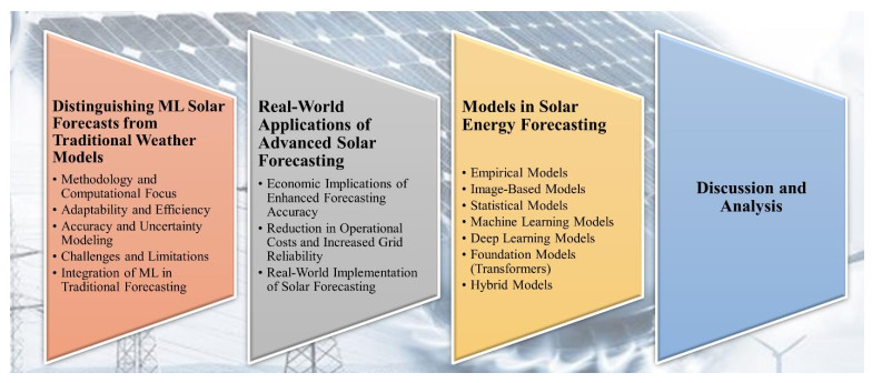
The need for accurate solar energy forecasting is paramount as the global push towards renewable energy intensifies. We aimed to provide a comprehensive analysis of the latest advancements in solar energy forecasting, focusing on Machine Learning (ML) and Deep Learning (DL) techniques. The novelty of this review lies in its detailed examination of ML and DL models, highlighting their ability to handle complex and nonlinear patterns in Solar Irradiance (SI) data. We systematically explored the evolution from traditional empirical, including machine learning (ML), and physical approaches to these advanced models, and delved into their real-world applications, discussing economic and policy implications. Additionally, we covered a variety of forecasting models, including empirical, image-based, statistical, ML, DL, foundation, and hybrid models. Our analysis revealed that ML and DL models significantly enhance forecasting accuracy, operational efficiency, and grid reliability, contributing to economic benefits and supporting sustainable energy policies. By addressing challenges related to data quality and model interpretability, this review underscores the importance of continuous innovation in solar forecasting techniques to fully realize their potential. The findings suggest that integrating these advanced models with traditional approaches offers the most promising path forward for improving solar energy forecasting.

| [1] |
EI Hendouzi A, Bourouhou A (2020) Solar Photovoltaic Power Forecasting. J Electr Comput Eng 2020: 1–21. https://doi.org/10.1155/2020/8819925 doi: 10.1155/2020/8819925

|
| [2] | Ürkmez M, Kallesøe C, Dimon Bendtsen J, et al. (2022) Day-ahead pv power forecasting for control applications. IECON 2022, 48th Annual Conference of the IEEE Industrial Electronics Society, Brussels, Belgium, 1–6. https://doi.org/10.1109/IECON49645.2022.9968709 |
| [3] |
Cheng S, Prentice IC, Huang Y, et al. (2022) Data-driven surrogate model with latent data assimilation: Application to wildfire forecasting. J Comput Phys 464: 111302. https://doi.org/10.1016/J.JCP.2022.111302 doi: 10.1016/J.JCP.2022.111302
|
| [4] |
Cheng S, Jin Y, Harrison SP, et al. (2022) Parameter Flexible Wildfire Prediction Using Machine Learning Techniques: Forward and Inverse Modelling. Remote Sens 14: 3228. https://doi.org/10.3390/RS14133228 doi: 10.3390/RS14133228
|
| [5] |
Zhong C, Cheng S, Kasoar M, et al. (2023) Reduced-order digital twin and latent data assimilation for global wildfire prediction. Nat Hazard Earth Sys 23: 1755–1768. https://doi.org/10.5194/NHESS-23-1755-2023 doi: 10.5194/NHESS-23-1755-2023
|
| [6] |
Gupta P, Singh R (2021) PV power forecasting based on data-driven models: a review. Int J Sustain Eng 14: 1733–1755. https://doi.org/10.1080/19397038.2021.1986590 doi: 10.1080/19397038.2021.1986590
|
| [7] |
López Santos M, García-Santiago X, Echevarría Camarero F, et al. (2022) Application of Temporal Fusion Transformer for Day-Ahead PV Power Forecasting. Energies 15: 5232. https://doi.org/10.3390/EN15145232 doi: 10.3390/EN15145232
|
| [8] | Kanchana W, Sirisukprasert S (2020) PV Power Forecasting with Holt-Winters Method. 2020 8th International Electrical Engineering Congress (IEECON), 1–4. https://doi.org/10.1109/IEECON48109.2020.229517 |
| [9] | Dhingra S, Gruosso G, Gajani GS (2023) Solar PV Power Forecasting and Ageing Evaluation Using Machine Learning Techniques. IECON 2023 49th Annual Conference of the IEEE Industrial Electronics Society, 1–6. https://doi.org/10.1109/IECON51785.2023.10312446 |
| [10] |
Hanif MF, Naveed MS, Metwaly M, et al. (2021) Advancing solar energy forecasting with modified ANN and light GBM learning algorithms. AIMS Energy 12: 350–386. https://doi.org/10.3934/ENERGY.2024017 doi: 10.3934/ENERGY.2024017
|
| [11] |
Hanif MF, Siddique MU, Si J, et al. (2021) Enhancing Solar Forecasting Accuracy with Sequential Deep Artificial Neural Network and Hybrid Random Forest and Gradient Boosting Models across Varied Terrains. Adv Theory Simul 7: 2301289. https://doi.org/10.1002/ADTS.202301289 doi: 10.1002/ADTS.202301289
|
| [12] | Musafa A, Priyadi A, Lystianingrum V, et al. (2023) Stored Energy Forecasting of Small-Scale Photovoltaic-Pumped Hydro Storage System Based on Prediction of Solar Irradiance, Ambient Temperature, and Rainfall Using LSTM Method. IECON 2023 49th Annual Conference of the IEEE Industrial Electronics, 1–6. https://doi.org/10.1109/IECON51785.2023.10311982 |
| [13] |
Konstantinou M, Peratikou S, Charalambides AG (2021) Solar Photovoltaic Forecasting of Power Output Using LSTM Networks. Atmosphere 12: 124. https://doi.org/10.3390/ATMOS12010124 doi: 10.3390/ATMOS12010124
|
| [14] | Jasiński M, Leonowicz Z, Jasiński J, et al. (2023) PV Advancements & Challenges: Forecasting Techniques, Real Applications, and Grid Integration for a Sustainable Energy Future. 2023 IEEE International Conference on Environment and Electrical Engineering and 2023 IEEE Industrial and Commercial Power Systems Europe (EEEIC/I & CPS Europe), Spain, 1–5. https://doi.org/10.1109/EEEIC/ICPSEUROPE57605.2023.10194796 |
| [15] |
Cantillo-Luna S, Moreno-Chuquen R, Celeita D, et al. (2023) Deep and Machine Learning Models to Forecast Photovoltaic Power Generation. Energies 16: 4097. https://doi.org/10.3390/EN16104097 doi: 10.3390/EN16104097
|
| [16] | Kaushik AR, Padmavathi S, Gurucharan KS, et al. (2023) Performance Analysis of Regression Models in Solar PV Forecasting. 2023 3rd International Conference on Artificial Intelligence and Signal Processing (AISP), India, 1–5. https://doi.org/10.1109/AISP57993.2023.10134943 |
| [17] |
Halabi LM, Mekhilef S, Hossain M (2018) Performance evaluation of hybrid adaptive neuro-fuzzy inference system models for predicting monthly global solar radiation. Appl Energy 213: 247–261. https://doi.org/10.1016/J.APENERGY.2018.01.035 doi: 10.1016/J.APENERGY.2018.01.035
|
| [18] |
Zhang G, Wang X, Du Z (2015) Research on the Prediction of Solar Energy Generation based on Measured Environmental Data. Int J U e-Service Sci Technol 8: 385–402. https://doi.org/10.14257/IJUNESST.2015.8.5.37 doi: 10.14257/IJUNESST.2015.8.5.37
|
| [19] | Peng Q, Zhou X, Zhu R, et al. (2023) A Hybrid Model for Solar Radiation Forecasting towards Energy Efficient Buildings. 2023 7th International Conference on Green Energy and Applications (ICGEA), 7–12. https://doi.org/10.1109/ICGEA57077.2023.10125987 |
| [20] | Salisu S, Mustafa MW, Mustapha M (2018) Predicting Global Solar Radiation in Nigeria Using Adaptive Neuro-Fuzzy Approach. Recent Trends in Information and Communication Technology. IRICT 2017. Lecture Notes on Data Engineering and Communications Technologies, 5: 513–521. https://doi.org/10.1007/978-3-319-59427-9_54 |
| [21] |
Kaur A, Nonnenmacher L, Pedro HTC, et al. (2016) Benefits of solar forecasting for energy imbalance markets. Renewable Energy 86: 819–830. https://doi.org/10.1016/J.RENENE.2015.09.011 doi: 10.1016/J.RENENE.2015.09.011
|
| [22] |
Yang D, Li W, Yagli GM, et al. (2021) Operational solar forecasting for grid integration: Standards, challenges, and outlook. Sol Energy 224: 930–937. https://doi.org/10.1016/J.SOLENER.2021.04.002 doi: 10.1016/J.SOLENER.2021.04.002
|
| [23] | Shi G, Eftekharnejad S (2016) Impact of solar forecasting on power system planning. 2016 North American Power Symposium (NAPS), 1–6. https://doi.org/10.1109/NAPS.2016.7747909 |
| [24] |
Shi J, Guo J, Zheng S (2012) Evaluation of hybrid forecasting approaches for wind speed and power generation time series. Renewable Sustainable Energy Rev 16: 3471–3480. https://doi.org/10.1016/j.rser.2012.02.044 doi: 10.1016/j.rser.2012.02.044
|
| [25] |
Mohanty S, Patra PK, Sahoo SS, et al. (2017) Forecasting of solar energy with application for a growing economy like India: Survey and implication. Renewable Sustainable Energy Rev 78: 539–553. https://doi.org/10.1016/J.RSER.2017.04.107 doi: 10.1016/J.RSER.2017.04.107
|
| [26] |
Sweeney C, Bessa RJ, Browell J, et al. (2020) The future of forecasting for renewable energy. Wiley Interdiscip Rev Energy Environ 9: e365. https://doi.org/10.1002/WENE.365 doi: 10.1002/WENE.365
|
| [27] |
Brancucci Martinez-Anido C, Botor B, Florita AR, et al. (2016) The value of day-ahead solar power forecasting improvement. Sol Energy 129: 192–203. https://doi.org/10.1016/J.SOLENER.2016.01.049 doi: 10.1016/J.SOLENER.2016.01.049
|
| [28] |
Inman RH, Pedro HTC, Coimbra CFM (2013) Solar forecasting methods for renewable energy integration. Prog Energy Combust Sci 39: 535–576. https://doi.org/10.1016/J.PECS.2013.06.002 doi: 10.1016/J.PECS.2013.06.002
|
| [29] |
Cui M, Zhang J, Hodge BM, et al. (2018) A Methodology for Quantifying Reliability Benefits from Improved Solar Power Forecasting in Multi-Timescale Power System Operations. IEEE T Smart Grid 9: 6897–6908. https://doi.org/10.1109/TSG.2017.2728480 doi: 10.1109/TSG.2017.2728480
|
| [30] |
Wang H, Lei Z, Zhang X, et al. (2019) A review of deep learning for renewable energy forecasting. Energy Convers Manage 198: 111799. https://doi.org/10.1016/J.ENCONMAN.2019.111799 doi: 10.1016/J.ENCONMAN.2019.111799
|
| [31] |
Aupke P, Kassler A, Theocharis A, et al. (2021) Quantifying Uncertainty for Predicting Renewable Energy Time Series Data Using Machine Learning. Eng Proc 5: 50. https://doi.org/10.3390/ENGPROC2021005050 doi: 10.3390/ENGPROC2021005050
|
| [32] |
Rajagukguk RA, Ramadhan RAA, Lee HJ (2020) A Review on Deep Learning Models for Forecasting Time Series Data of Solar Irradiance and Photovoltaic Power. Energies 13: 6623. https://doi.org/10.3390/EN13246623 doi: 10.3390/EN13246623
|
| [33] | SETO 2020—Artificial Intelligence Applications in Solar Energy. Available from: https://www.energy.gov/eere/solar/seto-2020-artificial-intelligence-applications-solar-energy. |
| [34] |
Freitas S, Catita C, Redweik P, et al. (2015) Modelling solar potential in the urban environment: State-of-the-art review. Renewable Sustainable Energy Rev 41: 915–931. https://doi.org/10.1016/J.RSER.2014.08.060 doi: 10.1016/J.RSER.2014.08.060
|
| [35] |
Gürtürk M, Ucar F, Erdem M (2022) A novel approach to investigate the effects of global warming and exchange rate on the solar power plants. Energy 239: 122344. https://doi.org/10.1016/J.ENERGY.2021.122344 doi: 10.1016/J.ENERGY.2021.122344
|
| [36] |
Gaye B, Zhang D, Wulamu A (2021) Improvement of Support Vector Machine Algorithm in Big Data Background. Math Probl Eng 2021: 5594899. https://doi.org/10.1155/2021/5594899 doi: 10.1155/2021/5594899
|
| [37] |
Yogambal Jayalakshmi N, Shankar R, Subramaniam U, et al. (2021) Novel Multi-Time Scale Deep Learning Algorithm for Solar Irradiance Forecasting. Energies 14: 2404. https://doi.org/10.3390/EN14092404 doi: 10.3390/EN14092404
|
| [38] |
Benti NE, Chaka MD, Semie AG (2023) Forecasting Renewable Energy Generation with Machine Learning and Deep Learning: Current Advances and Future Prospects. Sustainability 15: 7087. https://doi.org/10.3390/SU15097087 doi: 10.3390/SU15097087
|
| [39] |
Li J, Ward JK, Tong J, et al. (2016) Machine learning for solar irradiance forecasting of photovoltaic system. Renewable Energy 90: 542–553. https://doi.org/10.1016/J.RENENE.2015.12.069 doi: 10.1016/J.RENENE.2015.12.069
|
| [40] |
Long H, Zhang Z, Su Y (2014) Analysis of daily solar power prediction with data-driven approaches. Appl Energy 126: 29–37. https://doi.org/10.1016/J.APENERGY.2014.03.084 doi: 10.1016/J.APENERGY.2014.03.084
|
| [41] |
Jebli I, Belouadha FZ, Kabbaj MI, et al. (2021) Prediction of solar energy guided by pearson correlation using machine learning. Energy 224: 120109. https://doi.org/10.1016/J.ENERGY.2021.120109 doi: 10.1016/J.ENERGY.2021.120109
|
| [42] |
Khandakar A, Chowdhury MEH, Kazi MK, et al. (2019) Machine Learning Based Photovoltaics (PV) Power Prediction Using Different Environmental Parameters of Qatar. Energies 12: 2782. https://doi.org/10.3390/EN12142782 doi: 10.3390/EN12142782
|
| [43] |
Kim SG, Jung JY, Sim MK (2019) A Two-Step Approach to Solar Power Generation Prediction Based on Weather Data Using Machine Learning. Sustainability 11: 1501. https://doi.org/10.3390/SU11051501 doi: 10.3390/SU11051501
|
| [44] |
Gutiérrez L, Patiño J, Duque-Grisales E (2021) A Comparison of the Performance of Supervised Learning Algorithms for Solar Power Prediction. Energies 14: 4424. https://doi.org/10.3390/EN14154424 doi: 10.3390/EN14154424
|
| [45] |
Wang Z, Xu Z, Zhang Y, et al. (2020) Optimal Cleaning Scheduling for Photovoltaic Systems in the Field Based on Electricity Generation and Dust Deposition Forecasting. IEEE J Photovolt 10: 1126–1132. https://doi.org/10.1109/JPHOTOV.2020.2981810 doi: 10.1109/JPHOTOV.2020.2981810
|
| [46] |
Massaoudi M, Chihi I, Sidhom L, et al. (2021) An Effective Hybrid NARX-LSTM Model for Point and Interval PV Power Forecasting. IEEE Access 9: 36571–36588. https://doi.org/10.1109/ACCESS.2021.3062776 doi: 10.1109/ACCESS.2021.3062776
|
| [47] |
Arora I, Gambhir J, Kaur T (2021) Data Normalisation-Based Solar Irradiance Forecasting Using Artificial Neural Networks. Arab J Sci Eng 46: 1333–1343. https://doi.org/10.1007/S13369-020-05140-Y/METRICS doi: 10.1007/S13369-020-05140-Y/METRICS
|
| [48] |
Alipour M, Aghaei J, Norouzi M, et al. (2020) A novel electrical net-load forecasting model based on deep neural networks and wavelet transform integration. Energy 205: 118106. https://doi.org/10.1016/J.ENERGY.2020.118106 doi: 10.1016/J.ENERGY.2020.118106
|
| [49] |
Zolfaghari M, Golabi MR (2021) Modeling and predicting the electricity production in hydropower using conjunction of wavelet transform, long short-term memory and random forest models. Renewable Energy 170: 1367–1381. https://doi.org/10.1016/J.RENENE.2021.02.017 doi: 10.1016/J.RENENE.2021.02.017
|
| [50] |
Li FF, Wang SY, Wei JH (2018) Long term rolling prediction model for solar radiation combining empirical mode decomposition (EMD) and artificial neural network (ANN) techniques. J Renewable Sustainable Energy 10: 013704. https://doi.org/10.1063/1.4999240 doi: 10.1063/1.4999240
|
| [51] | Wang S, Guo Y, Wang Y, et al. (2021) A Wind Speed Prediction Method Based on Improved Empirical Mode Decomposition and Support Vector Machine. IOP Conference Series: Earth and Environmental Science, IOP Publishing. 680: 012012. https://doi.org/10.1088/1755-1315/680/1/012012 |
| [52] |
Moreno SR, dos Santos Coelho L (2018) Wind speed forecasting approach based on Singular Spectrum Analysis and Adaptive Neuro Fuzzy Inference System. Renewable Energy 126: 736–754. https://doi.org/10.1016/J.RENENE.2017.11.089 doi: 10.1016/J.RENENE.2017.11.089
|
| [53] |
Zhang Y, Le J, Liao X, et al. (2019) A novel combination forecasting model for wind power integrating least square support vector machine, deep belief network, singular spectrum analysis and locality-sensitive hashing. Energy 168: 558–572. https://doi.org/10.1016/J.ENERGY.2018.11.128 doi: 10.1016/J.ENERGY.2018.11.128
|
| [54] | Espinar B, Aznarte JL, Girard R, et al. (2010) Photovoltaic Forecasting: A state of the art. 5th European PV-hybrid and mini-grid conference. OTTI-Ostbayerisches Technologie-Transfer-Institut. |
| [55] | Moreno-Munoz A, De La Rosa JJG, Posadillo R, et al. (2008) Very short term forecasting of solar radiation. 2008 33rd IEEE Photovoltaic Specialists Conference, San Diego, CA, USA. https://doi.org/10.1109/PVSC.2008.4922587 |
| [56] |
Anderson D, Leach M (2004) Harvesting and redistributing renewable energy: on the role of gas and electricity grids to overcome intermittency through the generation and storage of hydrogen. Energy Policy 32: 1603–1614. https://doi.org/10.1016/S0301-4215(03)00131-9 doi: 10.1016/S0301-4215(03)00131-9
|
| [57] |
Zhang J, Zhao L, Deng S, et al. (2017) A critical review of the models used to estimate solar radiation. Renewable Sustainable Energy Rev 70: 314–329. https://doi.org/10.1016/J.RSER.2016.11.124 doi: 10.1016/J.RSER.2016.11.124
|
| [58] |
Coimbra CFM, Kleissl J, Marquez R (2013) Overview of Solar-Forecasting Methods and a Metric for Accuracy Evaluation. Sol Energy Forecast Resour Assess, 171–194. https://doi.org/10.1016/B978-0-12-397177-7.00008-5 doi: 10.1016/B978-0-12-397177-7.00008-5
|
| [59] |
Miller SD, Rogers MA, Haynes JM, et al. (2018) Short-term solar irradiance forecasting via satellite/model coupling. Sol Energy 168: 102–117. https://doi.org/10.1016/J.SOLENER.2017.11.049 doi: 10.1016/J.SOLENER.2017.11.049
|
| [60] |
Kumari P, Toshniwal D (2021) Deep learning models for solar irradiance forecasting: A comprehensive review. J Cleaner Prod 318: 128566. https://doi.org/10.1016/J.JCLEPRO.2021.128566 doi: 10.1016/J.JCLEPRO.2021.128566
|
| [61] |
Hassan GE, Youssef ME, Mohamed ZE, et al. (2016) New Temperature-based Models for Predicting Global Solar Radiation. Appl Energy 179: 437–450. https://doi.org/10.1016/J.APENERGY.2016.07.006 doi: 10.1016/J.APENERGY.2016.07.006
|
| [62] |
Angstrom A (1924) Solar and terrestrial radiation. Report to the international commission for solar research on actinometric investigations of solar and atmospheric radiation. Q J R Meteorol Soc 50: 121–126. https://doi.org/10.1002/QJ.49705021008 doi: 10.1002/QJ.49705021008
|
| [63] |
Samuel TDMA (1991) Estimation of global radiation for Sri Lanka. Sol Energy 47: 333–337. https://doi.org/10.1016/0038-092X(91)90026-S doi: 10.1016/0038-092X(91)90026-S
|
| [64] |
Ögelman H, Ecevit A, Tasdemiroǧlu E (1984) A new method for estimating solar radiation from bright sunshine data. Sol Energy 33: 619–625. https://doi.org/10.1016/0038-092X(84)90018-5 doi: 10.1016/0038-092X(84)90018-5
|
| [65] |
Badescu V, Gueymard CA, Cheval S, et al. (2013) Accuracy analysis for fifty-four clear-sky solar radiation models using routine hourly global irradiance measurements in Romania. Renewable Energy 55: 85–103. https://doi.org/10.1016/J.RENENE.2012.11.037 doi: 10.1016/J.RENENE.2012.11.037
|
| [66] |
Mecibah MS, Boukelia TE, Tahtah R, et al. (2014) Introducing the best model for estimation the monthly mean daily global solar radiation on a horizontal surface (Case study: Algeria). Renewable Sustainable Energy Rev 36: 194–202. https://doi.org/10.1016/J.RSER.2014.04.054 doi: 10.1016/J.RSER.2014.04.054
|
| [67] |
Hargreaves GH, Samani ZA (1982) Estimating Potential Evapotranspiration. J Irrig Drain Div 108: 225–230. https://doi.org/10.1061/JRCEA4.0001390 doi: 10.1061/JRCEA4.0001390
|
| [68] |
Bristow KL, Campbell GS (1984) On the relationship between incoming solar radiation and daily maximum and minimum temperature. Agric For Meteorol 31: 159–166. https://doi.org/10.1016/0168-1923(84)90017-0 doi: 10.1016/0168-1923(84)90017-0
|
| [69] |
Chen JL, He L, Yang H, et al. (2019) Empirical models for estimating monthly global solar radiation: A most comprehensive review and comparative case study in China. Renewable Sustainable Energy Rev 108: 91–111. https://doi.org/10.1016/j.rser.2019.03.033 doi: 10.1016/j.rser.2019.03.033
|
| [70] |
Chen Y, Zhang S, Zhang W, et al. (2019) Multifactor spatio-temporal correlation model based on a combination of convolutional neural network and long short-term memory neural network for wind speed forecasting. Energy Convers Manage 185: 783–799. https://doi.org/10.1016/j.enconman.2019.02.01 doi: 10.1016/j.enconman.2019.02.01
|
| [71] | Siddiqui TA, Bharadwaj S, Kalyanaraman S (2019) A Deep Learning Approach to Solar-Irradiance Forecasting in Sky-Videos. 2019 IEEE Winter Conference on Applications of Computer Vision (WACV), 2166–2174. https://doi.org/10.1109/WACV.2019.00234 |
| [72] |
Nie Y, Li X, Paletta Q, et al. (2024) Open-source sky image datasets for solar forecasting with deep learning: A comprehensive survey. Renewable Sustainable Energy Rev 189: 113977. https://doi.org/10.1016/j.rser.2023.113977 doi: 10.1016/j.rser.2023.113977
|
| [73] | SkyImageNet, 2024. Available from: https://github.com/SkyImageNet. |
| [74] |
Brahma B, Wadhvani R (2020) Solar Irradiance Forecasting Based on Deep Learning Methodologies and Multi-Site Data. Symmetry 12: 1–20. https://doi.org/10.3390/sym12111830 doi: 10.3390/sym12111830
|
| [75] |
Paletta Q, Terrén-Serrano G, Nie Y, et al. (2023) Advances in solar forecasting: Computer vision with deep learning. Adv Appl Energy 11: 100150. https://doi.org/10.1016/j.adapen.2023.100150 doi: 10.1016/j.adapen.2023.100150
|
| [76] |
Ghimire S, Deo RC, Raj N, et al. (2019) Deep solar radiation forecasting with convolutional neural network and long short-term memory network algorithms. Appl Energy 253: 113541. https://doi.org/10.1016/J.APENERGY.2019.113541 doi: 10.1016/J.APENERGY.2019.113541
|
| [77] |
Elsaraiti M, Merabet A (2022) Solar Power Forecasting Using Deep Learning Techniques. IEEE Access 10: 31692–31698. https://doi.org/10.1109/ACCESS.2022.3160484 doi: 10.1109/ACCESS.2022.3160484
|
| [78] |
Reikard G (2009) Predicting solar radiation at high resolutions: A comparison of time series forecasts. Sol Energy 83: 342–349. https://doi.org/10.1016/J.SOLENER.2008.08.007 doi: 10.1016/J.SOLENER.2008.08.007
|
| [79] |
Yang D, Jirutitijaroen P, Walsh WM (2012) Hourly solar irradiance time series forecasting using cloud cover index. Sol Energy 86: 3531–3543. https://doi.org/10.1016/J.SOLENER.2012.07.029 doi: 10.1016/J.SOLENER.2012.07.029
|
| [80] |
Jaihuni M, Basak JK, Khan F, et al. (2020) A Partially Amended Hybrid Bi-GRU—ARIMA Model (PAHM) for Predicting Solar Irradiance in Short and Very-Short Terms. Energies 13: 435. https://doi.org/10.3390/EN13020435 doi: 10.3390/EN13020435
|
| [81] |
Verbois H, Huva R, Rusydi A, et al. (2018) Solar irradiance forecasting in the tropics using numerical weather prediction and statistical learning. Sol Energy 162: 265–277. https://doi.org/10.1016/j.solener.2018.01.007 doi: 10.1016/j.solener.2018.01.007
|
| [82] |
Munkhammar J, van der Meer D, Widén J (2019) Probabilistic forecasting of high-resolution clear-sky index time-series using a Markov-chain mixture distribution model. Sol Energy 184: 688–695. https://doi.org/10.1016/j.solener.2019.04.014 doi: 10.1016/j.solener.2019.04.014
|
| [83] |
Dong J, Olama MM, Kuruganti T, et al. (2020) Novel stochastic methods to predict short-term solar radiation and photovoltaic power. Renewable Energy 145: 333–346. https://doi.org/10.1016/j.renene.2019.05.073 doi: 10.1016/j.renene.2019.05.073
|
| [84] |
Ahmad T, Zhang D, Huang C (2021) Methodological framework for short-and medium-term energy, solar and wind power forecasting with stochastic-based machine learning approach to monetary and energy policy applications. Energy 231: 120911. https://doi.org/10.1016/j.energy.2021.120911 doi: 10.1016/j.energy.2021.120911
|
| [85] | Box GE, Jenkins GM, Reinsel GC, et al. (2015) Time series analysis: Forecasting and control, John Wiley & Sons. |
| [86] |
Louzazni M, Mosalam H, Khouya A (2020) A non-linear auto-regressive exogenous method to forecast the photovoltaic power output. Sustain Energy Techn 38: 100670. https://doi.org/10.1016/j.seta.2020.100670 doi: 10.1016/j.seta.2020.100670
|
| [87] |
Larson DP, Nonnenmacher L, Coimbra CFM (2016) Day-ahead forecasting of solar power output from photovoltaic plants in the American Southwest. Renewable Energy 91: 11–20. https://doi.org/10.1016/j.renene.2016.01.039 doi: 10.1016/j.renene.2016.01.039
|
| [88] |
Sharma V, Yang D, Walsh W, et al. (2016) Short term solar irradiance forecasting using a mixed wavelet neural network. Renewable Energy 90: 481–492. https://doi.org/10.1016/J.RENENE.2016.01.020 doi: 10.1016/J.RENENE.2016.01.020
|
| [89] | Kumari P, Toshniwal D (2020) Real-time estimation of COVID-19 cases using machine learning and mathematical models-The case of India. 2020 IEEE 15th International Conference on Industrial and Information Systems, 369–374. https://doi.org/10.1109/ICIIS51140.2020.9342735 |
| [90] |
Ahmad MW, Mourshed M, Rezgui Y (2018) Tree-based ensemble methods for predicting PV power generation and their comparison with support vector regression. Energy 164: 465–474. https://doi.org/10.1016/J.ENERGY.2018.08.207 doi: 10.1016/J.ENERGY.2018.08.207
|
| [91] |
Wang Z, Wang Y, Zeng R, et al. (2018) Random Forest based hourly building energy prediction. Energy Buildings 171: 11–25. https://doi.org/10.1016/J.ENBUILD.2018.04.008 doi: 10.1016/J.ENBUILD.2018.04.008
|
| [92] |
Zou L, Wang L, Lin A, et al. (2016) Estimation of global solar radiation using an artificial neural network based on an interpolation technique in southeast China. J Atmos Sol-Terr Phys 146: 110–122. https://doi.org/10.1016/J.JASTP.2016.05.013 doi: 10.1016/J.JASTP.2016.05.013
|
| [93] |
Mellit A, Benghanem M, Kalogirou SA (2006) An adaptive wavelet-network model for forecasting daily total solar-radiation. Appl Energy 83: 705–722. https://doi.org/10.1016/J.APENERGY.2005.06.003 doi: 10.1016/J.APENERGY.2005.06.003
|
| [94] |
Çelik Ö, Teke A, Yildirim HB (2016) The optimized artificial neural network model with Levenberg–Marquardt algorithm for global solar radiation estimation in Eastern Mediterranean Region of Turkey. J Cleaner Prod 116: 1–12. https://doi.org/10.1016/J.JCLEPRO.2015.12.082 doi: 10.1016/J.JCLEPRO.2015.12.082
|
| [95] |
Rehman S, Mohandes M (2008) Artificial neural network estimation of global solar radiation using air temperature and relative humidity. Energy Policy 36: 571–576. https://doi.org/10.1016/J.ENPOL.2007.09.033 doi: 10.1016/J.ENPOL.2007.09.033
|
| [96] |
Gürel AE, Ağbulut Ü, Biçen Y (2020) Assessment of machine learning, time series, response surface methodology and empirical models in prediction of global solar radiation. J Cleaner Prod 277: 122353. https://doi.org/10.1016/J.JCLEPRO.2020.122353 doi: 10.1016/J.JCLEPRO.2020.122353
|
| [97] |
Díaz-Gómez J, Parrales A, Á lvarez A, et al. (2015) Prediction of global solar radiation by artificial neural network based on a meteorological environmental data. Desalin Water Treat 55: 3210–3217. https://doi.org/10.1080/19443994.2014.939861 doi: 10.1080/19443994.2014.939861
|
| [98] |
Rocha PAC, Fernandes JL, Modolo AB, et al. (2019) Estimation of daily, weekly and monthly global solar radiation using ANNs and a long data set: a case study of Fortaleza, in Brazilian Northeast region. Int J Energy Environ Eng 10: 319–334. https://doi.org/10.1007/S40095-019-0313-0/TABLES/6 doi: 10.1007/S40095-019-0313-0/TABLES/6
|
| [99] |
Rezrazi A, Hanini S, Laidi M (2016) An optimisation methodology of artificial neural network models for predicting solar radiation: a case study. Theor Appl Climatol 123: 769–783. https://doi.org/10.1007/s00704-015-1398-x doi: 10.1007/s00704-015-1398-x
|
| [100] |
Pang Z, Niu F, O'Neill Z (2020) Solar radiation prediction using recurrent neural network and artificial neural network: A case study with comparisons. Renewable Energy 156: 279–289. https://doi.org/10.1016/J.RENENE.2020.04.042 doi: 10.1016/J.RENENE.2020.04.042
|
| [101] |
Toth E, Brath A, Montanari A (2000) Comparison of short-term rainfall prediction models for real-time flood forecasting. J Hydrol 239: 132–147. https://doi.org/10.1016/S0022-1694(00)00344-9 doi: 10.1016/S0022-1694(00)00344-9
|
| [102] | Mamoulis N, Seidl T, Pedersen TB, et al. (2009) Advances in Spatial and Temporal Databases, Springer Berlin, Heidelberg. https://doi.org/10.1007/978-3-642-02982-0 |
| [103] |
Ren J, Ren B, Zhang Q, et al. (2019) A Novel Hybrid Extreme Learning Machine Approach Improved by K Nearest Neighbor Method and Fireworks Algorithm for Flood Forecasting in Medium and Small Watershed of Loess Region. Water 11: 1848. https://doi.org/10.3390/W11091848 doi: 10.3390/W11091848
|
| [104] | Larose DT, Larose CD (2014) k‐Nearest Neighbor Algorithm. Discovering Knowledge in Data: An Introduction to Data Mining, Second Edition, 149–164. https://doi.org/10.1002/9781118874059.CH7 |
| [105] |
Sutton C (2012) Nearest-neighbor methods. WIREs Comput Stat 4: 307–309. https://doi.org/10.1002/WICS.1195 doi: 10.1002/WICS.1195
|
| [106] |
Chen JL, Li GS, Xiao BB, et al. (2015) Assessing the transferability of support vector machine model for estimation of global solar radiation from air temperature. Energy Convers Manage 89: 318–329. https://doi.org/10.1016/j.enconman.2014.10.004 doi: 10.1016/j.enconman.2014.10.004
|
| [107] | Shamshirband S, Mohammadi K, Tong CW, et al. (2016) A hybrid SVM-FFA method for prediction of monthly mean global solar radiation. Theor Appl Climatol 125: 53–65. |
| [108] |
Olatomiwa L, Mekhilef S, Shamshirband S, et al. (2015) Potential of support vector regression for solar radiation prediction in Nigeria. Nat Hazards 77: 1055–1068. https://doi.org/10.1007/s11069-015-1641-x doi: 10.1007/s11069-015-1641-x
|
| [109] |
Ramedani Z, Omid M, Keyhani A, et al. (2014) Potential of radial basis function based support vector regression for global solar radiation prediction. Renewable Sustainable Energy Rev 39: 1005–1011. https://doi.org/10.1016/J.RSER.2014.07.108 doi: 10.1016/J.RSER.2014.07.108
|
| [110] |
Olatomiwa L, Mekhilef S, Shamshirband S, et al. (2015) A support vector machine-firefly algorithm-based model for global solar radiation prediction. Sol Energy 115: 632–644. https://doi.org/10.1016/j.solener.2015.03.015 doi: 10.1016/j.solener.2015.03.015
|
| [111] |
Mohammadi K, Shamshirband S, Danesh AS, et al. (2016) Temperature-based estimation of global solar radiation using soft computing methodologies. Theor Appl Climatol 125: 101–112. https://doi.org/10.1007/s00704-015-1487-x doi: 10.1007/s00704-015-1487-x
|
| [112] |
Hassan MA, Khalil A, Kaseb S, et al. (2017) Potential of four different machine-learning algorithms in modeling daily global solar radiation. Renewable Energy 111: 52–62. https://doi.org/10.1016/j.renene.2017.03.083 doi: 10.1016/j.renene.2017.03.083
|
| [113] |
Quej VH, Almorox J, Arnaldo JA, et al. (2017) ANFIS, SVM and ANN soft-computing techniques to estimate daily global solar radiation in a warm sub-humid environment. J Atmos Sol-Terr Phys 155: 62–70. https://doi.org/10.1016/J.JASTP.2017.02.002 doi: 10.1016/J.JASTP.2017.02.002
|
| [114] |
Baser F, Demirhan H (2017) A fuzzy regression with support vector machine approach to the estimation of horizontal global solar radiation. Energy 123: 229–240. https://doi.org/10.1016/j.energy.2017.02.008 doi: 10.1016/j.energy.2017.02.008
|
| [115] |
Breiman L (2001) Random forests. Mach Learn 45: 5–32. https://doi.org/10.1023/A:1010933404324 doi: 10.1023/A:1010933404324
|
| [116] | Fernández-Delgado M, Cernadas E, Barro S, et al. (2014) Do we need hundreds of classifiers to solve real world classification problems? J Mach Learn Res 15: 3133–3181. |
| [117] | Ke G, Meng Q, Finley T, et al. (2017) Lightgbm: A highly efficient gradient boosting decision tree. Adv Neural Inf Proc Syst, 30. |
| [118] |
Wang Y, Pan Z, Zheng J, et al. (2019) A hybrid ensemble method for pulsar candidate classification. Astrophys Space Sci 364: 139 https://doi.org/10.1007/s10509-019-3602-4 doi: 10.1007/s10509-019-3602-4
|
| [119] |
Si Z, Yang M, Yu Y, et al. (2021) Photovoltaic power forecast based on satellite images considering effects of solar position. Appl Energy 302: 117514. https://doi.org/10.1016/j.apenergy.2021.117514 doi: 10.1016/j.apenergy.2021.117514
|
| [120] | Chung J, Gulcehre C, Cho K, et al. (2014) Empirical Evaluation of Gated Recurrent Neural Networks on Sequence Modeling. arXiv preprint arXiv: 1412.3555. |
| [121] |
Wang Y, Liao W, Chang Y (2018) Gated Recurrent Unit Network-Based Short-Term Photovoltaic Forecasting. Energies 11: 2163. https://doi.org/10.3390/EN11082163 doi: 10.3390/EN11082163
|
| [122] |
Pazikadin AR, Rifai D, Ali K, et al. (2020) Solar irradiance measurement instrumentation and power solar generation forecasting based on Artificial Neural Networks (ANN): A review of five years research trend. Sci Total Environ 715: 136848. https://doi.org/10.1016/j.scitotenv.2020.136848 doi: 10.1016/j.scitotenv.2020.136848
|
| [123] |
Wang F, Xuan Z, Zhen Z, et al. (2020) A day-ahead PV power forecasting method based on LSTM-RNN model and time correlation modification under partial daily pattern prediction framework. Energy Convers Manage 212: 112766. https://doi.org/10.1016/j.enconman.2020.112766 doi: 10.1016/j.enconman.2020.112766
|
| [124] |
Zhang J, Yan J, Infield D, et al. (2019) Short-term forecasting and uncertainty analysis of wind turbine power based on long short-term memory network and Gaussian mixture model. Appl Energy 241: 229–244. https://doi.org/10.1016/j.apenergy.2019.03.044 doi: 10.1016/j.apenergy.2019.03.044
|
| [125] |
Liu H, Mi X, Li Y, et al. (2019) Smart wind speed deep learning based multi-step forecasting model using singular spectrum analysis, convolutional Gated Recurrent Unit network and Support Vector Regression. Renewable Energy 143: 842–854. https://doi.org/10.1016/j.renene.2019.05.039 doi: 10.1016/j.renene.2019.05.039
|
| [126] |
Tealab A (2018) Time series forecasting using artificial neural networks methodologies: A systematic review. Future Comput Inf J 3: 334–340. https://doi.org/10.1016/j.fcij.2018.10.003 doi: 10.1016/j.fcij.2018.10.003
|
| [127] |
Dong N, Chang JF, Wu AG, et al. (2020) A novel convolutional neural network framework based solar irradiance prediction method. Int J Electr Power Energy Syst 114: 105411. https://doi.org/10.1016/j.ijepes.2019.105411 doi: 10.1016/j.ijepes.2019.105411
|
| [128] | Hinton GE, Srivastava N, Krizhevsky A, et al. (2012) Improving neural networks by preventing co-adaptation of feature detectors. |
| [129] |
Han Z, Zhao J, Leung H, et al. (2021) A Review of Deep Learning Models for Time Series Prediction. IEEE Sens J 21: 7833–7848. https://doi.org/10.1109/JSEN.2019.2923982 doi: 10.1109/JSEN.2019.2923982
|
| [130] | Shi X, Chen Z, Wang H, et al. (2015) Convolutional LSTM Network: A Machine Learning Approach for Precipitation Nowcasting. Adv Neural Inf Proc Syst, 28. |
| [131] | Oord A van den, Dieleman S, Zen H, et al. (2016) WaveNet: A Generative Model for Raw Audio. arXiv preprint arXiv: 1609.03499. https://doi.org/10.48550/arXiv.1609.03499 |
| [132] | Bai S, Kolter JZ, Koltun V (2018) An Empirical Evaluation of Generic Convolutional and Recurrent Networks for Sequence Modeling. https://doi.org/10.48550/arXiv.1803.01271 |
| [133] | Vaswani A, Brain G, Shazeer N, et al. (2017) Attention Is All You Need. arXiv preprint arXiv: 1706.03762. |
| [134] |
Zang H, Liu L, Sun L, et al. (2020) Short-term global horizontal irradiance forecasting based on a hybrid CNN-LSTM model with spatiotemporal correlations. Renewable Energy 160: 26–41. https://doi.org/10.1016/j.renene.2020.05.150 doi: 10.1016/j.renene.2020.05.150
|
| [135] |
Qu J, Qian Z, Pei Y (2021) Day-ahead hourly photovoltaic power forecasting using attention-based CNN-LSTM neural network embedded with multiple relevant and target variables prediction pattern. Energy 232: 120996. https://doi.org/10.1016/j.energy.2021.120996 doi: 10.1016/j.energy.2021.120996
|
| [136] |
Schmidhuber J, Hochreiter S (1997) Long Short-Term Memory. Neural Comput 9: 1735–1780. https://doi.org/10.1162/neco.1997.9.8.1735 doi: 10.1162/neco.1997.9.8.1735
|
| [137] |
Venkatraman A, Hebert M, Bagnell J (2015) Improving Multi-Step Prediction of Learned Time Series Models. Proceedings of the AAAI Conference on Artificial Intelligence, 29. https://doi.org/10.1609/aaai.v29i1.9590 doi: 10.1609/aaai.v29i1.9590
|
| [138] |
Muhammad, Kennedy J, Lim CW (2022) Machine learning and deep learning in phononic crystals and metamaterials—A review. Mater Today Commun 33: 104606. https://doi.org/10.1016/J.MTCOMM.2022.104606 doi: 10.1016/J.MTCOMM.2022.104606
|
| [139] |
Yao G, Lei T, Zhong J (2019) A review of Convolutional-Neural-Network-based action recognition. Pattern Recogn Lett 118: 14–22. https://doi.org/10.1016/J.PATREC.2018.05.018 doi: 10.1016/J.PATREC.2018.05.018
|
| [140] |
Akram MW, Li G, Jin Y, et al. (2019) CNN based automatic detection of photovoltaic cell defects in electroluminescence images. Energy 189: 116319. https://doi.org/10.1016/J.ENERGY.2019.116319 doi: 10.1016/J.ENERGY.2019.116319
|
| [141] |
Bejani MM, Ghatee M (2021) A systematic review on overfitting control in shallow and deep neural networks. Artif Intell Rev 54: 6391–6438. https://doi.org/10.1007/s10462-021-09975-1 doi: 10.1007/s10462-021-09975-1
|
| [142] |
McCann MT, Jin KH, Unser M (2017) Convolutional neural networks for inverse problems in imaging: A review. IEEE Signal Proc Mag 34: 85–95. https://doi.org/10.1109/MSP.2017.2739299 doi: 10.1109/MSP.2017.2739299
|
| [143] |
Qian C, Xu B, Chang L, et al. (2021) Convolutional neural network based capacity estimation using random segments of the charging curves for lithium-ion batteries. Energy 227: 120333. https://doi.org/10.1016/J.ENERGY.2021.120333 doi: 10.1016/J.ENERGY.2021.120333
|
| [144] |
Liu Y, Guan L, Hou C, et al. (2019) Wind Power Short-Term Prediction Based on LSTM and Discrete Wavelet Transform. Appl Sci 9: 1108. https://doi.org/10.3390/APP9061108 doi: 10.3390/APP9061108
|
| [145] |
Husein M, Chung IY (2019) Day-Ahead Solar Irradiance Forecasting for Microgrids Using a Long Short-Term Memory Recurrent Neural Network: A Deep Learning Approach. Energies 12: 1856. https://doi.org/10.3390/EN12101856 doi: 10.3390/EN12101856
|
| [146] |
Zhao Z, Chen W, Wu X, et al. (2017) LSTM network: a deep learning approach for short-term traffic forecast. IET Intell Transp Syst 11: 68–75. https://doi.org/10.1049/IET-ITS.2016.0208 doi: 10.1049/IET-ITS.2016.0208
|
| [147] |
Suresh V, Janik P, Rezmer J, et al. (2020) Forecasting Solar PV Output Using Convolutional Neural Networks with a Sliding Window Algorithm. Energies 13: 723. https://doi.org/10.3390/EN13030723 doi: 10.3390/EN13030723
|
| [148] |
Zameer A, Jaffar F, Shahid F, et al. (2023) Short-term solar energy forecasting: Integrated computational intelligence of LSTMs and GRU. PLoS One 18: e0285410. https://doi.org/10.1371/journal.pone.0285410 doi: 10.1371/journal.pone.0285410
|
| [149] | Bommasani R, Hudson DA, Adeli E, et al. (2021) On the Opportunities and Risks of Foundation Models. arXiv preprint arXiv: 2108.07258. https://doi.org/10.48550/arXiv.2108.07258 |
| [150] | Devlin J (2018) BERT: Pre-training of Deep Bidirectional Transformers for Language Understanding. arXiv preprint arXiv: 1810.04805. |
| [151] | Mann B, Ryder N, Subbiah M, et al. (2020) Language Models are Few-Shot Learners. arXiv preprint arXiv: 2005.14165, 1. |
| [152] | Radford A, Kim JW, Hallacy C, et al. (2021) Learning Transferable Visual Models from Natural Language Supervision. International conference on machine learning. PMLR. |
| [153] | Child R, Gray S, Radford A, et al. (2019) Generating Long Sequences with Sparse Transformers. arXiv preprint arXiv: 1904.10509. https://doi.org/10.48550/arXiv.1904.10509 |
| [154] | Kitaev N, Kaiser Ł, Levskaya A (2020) Reformer: The Efficient Transformer. arXiv preprint arXiv: 2001.04451. https://doi.org/10.48550/arXiv.2001.04451 |
| [155] | Beltagy I, Peters ME, Cohan A (2020) Longformer: The Long-Document Transformer. arXiv preprint arXiv: 2004.05150. https://doi.org/10.48550/arXiv.2004.05150 |
| [156] | Wang S, Li BZ, Khabsa M, et al. (2020) Linformer: Self-Attention with Linear Complexity. arXiv preprint arXiv: 2006.04768. https://doi.org/10.48550/arXiv.2006.04768 |
| [157] | Rae JW, Potapenko A, Jayakumar SM, et al. (2020) Compressive Transformers for Long-Range Sequence Modelling. arXiv preprint arXiv: 1911.05507. https://doi.org/10.48550/arXiv.1911.05507 |
| [158] | Dai Z, Yang Z, Yang Y, et al. (2019) Transformer-XL: Attentive Language Models Beyond a Fixed-Length Context. Proceedings of the 57th Annual Meeting of the Association for Computational Linguistics, 2978–2988, Florence, Italy. Association for Computational Linguistics. https://doi.org/10.18653/v1/p19-1285 |
| [159] |
Zhou H, Zhang S, Peng J, et al. (2021) Informer: Beyond Efficient Transformer for Long Sequence Time-Series Forecasting. Proceedings of the AAAI Conference on Artificial Intelligence, 35: 11106–11115. https://doi.org/10.1609/AAAI.V35I12.17325 doi: 10.1609/AAAI.V35I12.17325
|
| [160] |
Hanif MF, Mi J (2024) Harnessing AI for solar energy: Emergence of transformer models. Appl Energy 369: 123541. https://doi.org/10.1016/J.APENERGY.2024.123541 doi: 10.1016/J.APENERGY.2024.123541
|
| [161] |
Hussain A, Khan ZA, Hussain T, et al. (2022) A Hybrid Deep Learning-Based Network for Photovoltaic Power Forecasting. Complexity. https://doi.org/10.1155/2022/7040601 doi: 10.1155/2022/7040601
|
| [162] |
Vennila C, Titus A, Sudha TS, et al. (2022) Forecasting Solar Energy Production Using Machine Learning. Int J Photoenergy 2022: 7797488. https://doi.org/10.1155/2022/7797488 doi: 10.1155/2022/7797488
|
| [163] |
So D, Oh J, Leem S, et al. (2023) A Hybrid Ensemble Model for Solar Irradiance Forecasting: Advancing Digital Models for Smart Island Realization. Electronics 12: 2607. https://doi.org/10.3390/electronics12122607 doi: 10.3390/electronics12122607
|
| [164] |
He Y, Liu Y, Shao S, et al. (2019) Application of CNN-LSTM in Gradual Changing Fault Diagnosis of Rod Pumping System. Math Probl Eng 2019: 4203821. https://doi.org/10.1155/2019/4203821 doi: 10.1155/2019/4203821
|
| [165] |
Huang CJ, Kuo PH (2018) A Deep CNN-LSTM Model for Particulate Matter (PM2.5) Forecasting in Smart Cities. Sensors 18: 2220. https://doi.org/10.3390/S18072220 doi: 10.3390/S18072220
|
| [166] |
Cao K, Kim H, Hwang C, et al. (2018) CNN-LSTM Coupled Model for Prediction of Waterworks Operation Data. J Inf Process Syst 14: 1508–1520. https://doi.org/10.3745/JIPS.02.0104 doi: 10.3745/JIPS.02.0104
|
| [167] |
Swapna G, Soman KP, Vinayakumar R (2018) Automated detection of diabetes using CNN and CNN-LSTM network and heart rate signals. Procedia Comput Sci 132: 1253–1262. https://doi.org/10.1016/j.procs.2018.05.041 doi: 10.1016/j.procs.2018.05.041
|
| [168] |
Jalali SMJ, Ahmadian S, Kavousi-Fard A, et al. (2022) Automated Deep CNN-LSTM Architecture Design for Solar Irradiance Forecasting. IEEE Trans Syst Man Cybernetics Syst 52: 54–65. https://doi.org/10.1109/TSMC.2021.3093519 doi: 10.1109/TSMC.2021.3093519
|
| [169] |
Lim SC, Huh JH, Hong SH, et al. (2022) Solar Power Forecasting Using CNN-LSTM Hybrid Model. Energies 15: 8233. https://doi.org/10.3390/EN15218233 doi: 10.3390/EN15218233
|
| [170] |
Covas E (2020) Transfer Learning in Spatial-Temporal Forecasting of the Solar Magnetic Field. Astron Nachr 341: 384–394. https://doi.org/10.1002/ASNA.202013690 doi: 10.1002/ASNA.202013690
|
| [171] |
Sheng H, Ray B, Chen K, et al. (2020) Solar Power Forecasting Based on Domain Adaptive Learning. IEEE Access 8: 198580–198590. https://doi.org/10.1109/ACCESS.2020.3034100 doi: 10.1109/ACCESS.2020.3034100
|
| [172] |
Ren X, Wang Y, Cao Z, et al. (2023) Feature Transfer and Rapid Adaptation for Few-Shot Solar Power Forecasting. Energies 16: 6211. https://doi.org/10.3390/EN16176211 doi: 10.3390/EN16176211
|
| [173] | Zhou S, Zhou L, Mao M, et al. (2020) Transfer Learning for Photovoltaic Power Forecasting with Long Short-Term Memory Neural Network. 2020 IEEE International Conference on Big Data and Smart Computing (BigComp), Busan, Korea (South), 125–132. https://doi.org/10.1109/BIGCOMP48618.2020.00-87 |
| [174] | Soleymani S, Mohammadzadeh S (2023) Comparative Analysis of Machine Learning Algorithms for Solar Irradiance Forecasting in Smart Grids. arXiv preprint arXiv: 2310.13791. https://doi.org/10.48550/arXiv.2310.13791 |
| [175] | Sutarna N, Tjahyadi C, Oktivasari P, et al. (2023) Machine Learning Algorithm and Modeling in Solar Irradiance Forecasting. 2023 6th International Conference of Computer and Informatics Engineering (IC2IE), Lombok, Indonesia, 221–225. https://doi.org/10.1109/IC2IE60547.2023.10330942 |
| [176] |
Bamisile O, Oluwasanmi A, Ejiyi C, et al. (2022) Comparison of machine learning and deep learning algorithms for hourly global/diffuse solar radiation predictions. Int J Energy Res 46: 10052–10073. https://doi.org/10.1002/ER.6529 doi: 10.1002/ER.6529
|
| [177] | Sahaya Lenin D, Teja Reddy R, Velaga V (2023) Solar Irradiance Forecasting Using Machine Learning. 2023 14th International Conference on Computing Communication and Networking Technologies (ICCCNT), Delhi, India, 1–7. https://doi.org/10.1109/ICCCNT56998.2023.10307660 |
| [178] |
Syahab AS, Hermawan A, Avianto D (2023) Global Horizontal Irradiance Prediction using the Algorithm of Moving Average and Exponential Smoothing. JISA 6: 74–81. https://doi.org/10.31326/JISA.V6I1.1649. doi: 10.31326/JISA.V6I1.1649
|
| [179] |
Aljanad A, Tan NML, Agelidis VG, et al. (2021) Neural Network Approach for Global Solar Irradiance Prediction at Extremely Short-Time-Intervals Using Particle Swarm Optimization Algorithm. Energies 14: 1213. https://doi.org/10.3390/EN14041213 doi: 10.3390/EN14041213
|
| [180] |
Mbah OM, Madueke CI, Umunakwe R, et al. (2022) Extreme Gradient Boosting: A Machine Learning Technique for Daily Global Solar Radiation Forecasting on Tilted Surfaces. J Eng Sci 9: E1–E6. https://doi.org/10.21272/JES.2022.9(2).E1 doi: 10.21272/JES.2022.9(2).E1
|
| [181] |
Cha J, Kim MK, Lee S, et al. (2021) Investigation of Applicability of Impact Factors to Estimate Solar Irradiance: Comparative Analysis Using Machine Learning Algorithms. Appl Sci 11: 8533. https://doi.org/10.3390/APP11188533 doi: 10.3390/APP11188533
|
| [182] | Reddy KR, Ray PK (2022) Solar Irradiance Forecasting using FFNN with MIG Feature Selection Technique. 2022 International Conference on Intelligent Controller and Computing for Smart Power (ICICCSP), Hyderabad, India, 01–05. https://doi.org/10.1109/ICICCSP53532.2022.9862335 |
| [183] |
Chandola D, Gupta H, Tikkiwal VA, et al. (2020) Multi-step ahead forecasting of global solar radiation for arid zones using deep learning. Procedia Comput Sci 167: 626–635. https://doi.org/10.1016/j.procs.2020.03.329 doi: 10.1016/j.procs.2020.03.329
|
| [184] |
Yang Y, Tang Z, Li Z, et al. (2023) Dual-Path Information Fusion and Twin Attention-Driven Global Modeling for Solar Irradiance Prediction. Sensors 23: 7649. https://doi.org/10.3390/S23177469 doi: 10.3390/S23177469
|
| [185] |
Meng F, Zou Q, Zhang Z, et al. (2021) An intelligent hybrid wavelet-adversarial deep model for accurate prediction of solar power generation. Energy Rep 7: 2155–2164. https://doi.org/10.1016/J.EGYR.2021.04.019 doi: 10.1016/J.EGYR.2021.04.019
|
| [186] | Kartini UT, Hariyati, Aribowo W, et al. (2022) Development Hybrid Model Deep Learning Neural Network (DL-NN) For Probabilistic Forecasting Solar Irradiance on Solar Cells To Improve Economics Value Added. 2022 Fifth International Conference on Vocational Education and Electrical Engineering (ICVEE), Surabaya, Indonesia, 151–156. https://doi.org/10.1109/ICVEE57061.2022.9930352 |
| [187] |
Singla P, Duhan M, Saroha S (2022) A dual decomposition with error correction strategy based improved hybrid deep learning model to forecast solar irradiance. Energy Sources Part A 44: 1583–1607. https://doi.org/10.1080/15567036.2022.2056267 doi: 10.1080/15567036.2022.2056267
|
| [188] |
Marinho FP, Rocha PAC, Neto ARR, et al. (2023) Short-Term Solar Irradiance Forecasting Using CNN-1D, LSTM and CNN-LSTM Deep Neural Networks: A Case Study with the Folsom (USA) Dataset. J Sol Energy Eng 145: 041002. https://doi.org/10.1115/1.4056122 doi: 10.1115/1.4056122
|
| [189] |
Kumari P, Toshniwal D (2021) Long short term memory-convolutional neural network based deep hybrid approach for solar irradiance forecasting. Appl Energy 295: 117061. https://doi.org/10.1016/j.apenergy.2021.117061 doi: 10.1016/j.apenergy.2021.117061
|
| [190] |
Elizabeth Michael N, Mishra M, Hasan S, et al. (2022) Short-Term Solar Power Predicting Model Based on Multi-Step CNN Stacked LSTM Technique. Energies 15: 2150. https://doi.org/10.3390/EN15062150 doi: 10.3390/EN15062150
|
| [191] |
Srivastava RK, Gupta A (2023) Short term solar irradiation forecasting using Deep neural network with decomposition methods and optimized by grid search algorithm. E3S Web Conf 405. https://doi.org/10.1051/E3SCONF/202340502011 doi: 10.1051/E3SCONF/202340502011
|
| [192] |
Ziyabari S, Zhao Z, Du L, et al. (2023) Multi-Branch ResNet-Transformer for Short-Term Spatio-Temporal Solar Irradiance Forecasting. IEEE Trans Ind Appl 59: 5293–5303. https://doi.org/10.1109/TIA.2023.3285202 doi: 10.1109/TIA.2023.3285202
|
| [193] |
Carneiro TC, De Carvalho PCM, Dos Santos HA, et al. (2022) Review on Photovoltaic Power and Solar Resource Forecasting: Current Status and Trends. J Sol Energy Eng 144: 010801. https://doi.org/10.1115/1.4051652 doi: 10.1115/1.4051652
|
| [194] |
Chaibi M, Benghoulam ELM, Tarik L, et al. (2021) An Interpretable Machine Learning Model for Daily Global Solar Radiation Prediction. Energies 14: 7367. https://doi.org/10.3390/EN14217367 doi: 10.3390/EN14217367
|
| [195] |
Mason L, González AB de, García-Closas M, et al. (2023) Interpretable, non-mechanistic forecasting using empirical dynamic modeling and interactive visualization. PLoS One 18: e0277149. https://doi.org/10.1101/2022.10.21.22281384 doi: 10.1101/2022.10.21.22281384
|
| [196] |
Rafati A, Joorabian M, Mashhour E, et al. (2021) High dimensional very short-term solar power forecasting based on a data-driven heuristic method. Energy 219: 119647. https://doi.org/10.1016/J.ENERGY.2020.119647 doi: 10.1016/J.ENERGY.2020.119647
|
| [197] |
Wang H, Cai R, Zhou B, et al. (2020) Solar irradiance forecasting based on direct explainable neural network. Energy Convers Manage 226: 113487. https://doi.org/10.1016/J.ENCONMAN.2020.113487 doi: 10.1016/J.ENCONMAN.2020.113487
|
| [198] |
Theocharides S, Makrides G, Livera A, et al. (2020) Day-ahead photovoltaic power production forecasting methodology based on machine learning and statistical post-processing. Appl Energy 268: 115023. https://doi.org/10.1016/J.APENERGY.2020.115023 doi: 10.1016/J.APENERGY.2020.115023
|


Figures(12) / Tables(3)

Ayesha Nadeem, Muhammad Farhan Hanif, Muhammad Sabir Naveed, Muhammad Tahir Hassan, Mustabshirha Gul, Naveed Husnain, Jianchun Mi. AI-Driven precision in solar forecasting: Breakthroughs in machine learning and deep learning[J]. AIMS Geosciences, 2024, 10(4): 684-734. doi: 10.3934/geosci.2024035


 DownLoad: