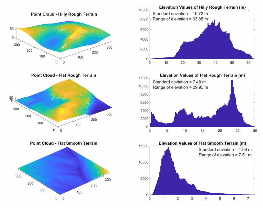
Terrain surface roughness, often described abstractly, poses challenges in quantitative characterization with various descriptors found in the literature. In this study, we compared five commonly used roughness descriptors, exploring correlations among their quantified terrain surface roughness maps across three terrains with distinct spatial variations. Additionally, we investigated the impacts of spatial scales and interpolation methods on these correlations. Dense point cloud data obtained through Light Detection and Ranging technique were used in this study. The findings highlighted both global pattern similarities and local pattern distinctions in the derived roughness maps, emphasizing the significance of incorporating multiple descriptors in studies where local roughness values play a crucial role in subsequent analyses. The spatial scales were found to have a smaller impact on rougher terrain, while interpolation methods had minimal influence on roughness maps derived from different descriptors.
Citation: Lei Fan, Yang Zhao. Comparing roughness maps generated by five typical roughness descriptors for LiDAR-derived digital elevation models[J]. AIMS Geosciences, 2024, 10(2): 228-241. doi: 10.3934/geosci.2024013
Terrain surface roughness, often described abstractly, poses challenges in quantitative characterization with various descriptors found in the literature. In this study, we compared five commonly used roughness descriptors, exploring correlations among their quantified terrain surface roughness maps across three terrains with distinct spatial variations. Additionally, we investigated the impacts of spatial scales and interpolation methods on these correlations. Dense point cloud data obtained through Light Detection and Ranging technique were used in this study. The findings highlighted both global pattern similarities and local pattern distinctions in the derived roughness maps, emphasizing the significance of incorporating multiple descriptors in studies where local roughness values play a crucial role in subsequent analyses. The spatial scales were found to have a smaller impact on rougher terrain, while interpolation methods had minimal influence on roughness maps derived from different descriptors.

| [1] |
Fernando JA, Francisco A, Manuel AA, et al. (2005) Effects of terrain morphology, sampling density, and interpolation methods on grid DEM accuracy. Photogramm Eng Remote Sens 71: 805–816. https://doi.org/10.14358/pers.71.7.805 doi: 10.14358/pers.71.7.805

|
| [2] |
Grohmann CH, Smith MJ, Riccomini C (2011) Multiscale analysis of topographic surface roughness in the Midland Valley, Scotland. IEEE Trans Geosci Remote Sens 49: 1200–1213. https://doi.org/10.1109/tgrs.2010.2053546 doi: 10.1109/tgrs.2010.2053546
|
| [3] |
Peter JB, Vernon HS, Jiro S, et al. (2004) Methods for Remote Engineering Geology Terrain Analysis in Boreal Forest Regions of Ontario, Canada. Environ Eng Geosci 10: 229–241. https://doi.org/10.2113/10.3.229 doi: 10.2113/10.3.229
|
| [4] |
Fan L, Atkinson PM (2015) Accuracy of digital elevation models derived from terrestrial laser scanning data. IEEE Geosci Remote Sens Lett 12: 1923-1927. https://doi.org/10.1109/LGRS.2015.2438394 doi: 10.1109/LGRS.2015.2438394
|
| [5] | Fan L (2014) Uncertainty in terrestrial laser scanning for measuring surface movements at a local scale. University of Southampton: Southampton, UK. |
| [6] |
Fan L, Powrie W, Smethurst JA, et al. (2014) The effect of short ground vegetation on terrestrial laser scans at a local scale. ISPRS J Photogramm Remote Sens 95: 42–52. https://doi.org/10.1016/j.isprsjprs.2014.06.003 doi: 10.1016/j.isprsjprs.2014.06.003
|
| [7] |
Frankel KL, Dolan JF (2007) Characterizing arid region alluvial fan surface roughness with airborne laser swath mapping digital topographic data. J Geophys Res 112: F02025. https://doi.org/10.1029/2006JF000644 doi: 10.1029/2006JF000644
|
| [8] |
Nield JM, Wiggs GFS (2011) The application of terrestrial laser scanning to aeolian saltation cloud measurement and its response to changing surface moisture. Earth Surf Processes Landforms 36: 273–278. https://doi.org/10.1002/esp.2102 doi: 10.1002/esp.2102
|
| [9] |
Kristen MB, Wayne LM, Patrick JD, et al. (2013) The Use of LiDAR Terrain Data in Characterizing Surface Roughness and Microtopography. Appl Environ Soil Sci 2013: 891534. https://doi.org/10.1155/2013/891534 doi: 10.1155/2013/891534
|
| [10] |
Milenković M, Pfeifer N, Glira P (2015) Applying Terrestrial Laser Scanning for Soil Surface Roughness Assessment. Remote Sens 7: 2007–2045. https://doi.org/10.3390/rs70202007 doi: 10.3390/rs70202007
|
| [11] |
Fan L (2020) A comparison between structure-from-motion and terrestrial laser scanning for deriving surface roughness: A case study on a sandy terrain surface. Int Arch Photogramm Remote Sens Spatial Inf Sci 42: 1225–1229. https://doi.org/10.5194/isprs-archives-XLⅡ-3-W10-1225-2020 doi: 10.5194/isprs-archives-XLⅡ-3-W10-1225-2020
|
| [12] |
Glenn NF, Streutker DR, Chadwick DJ, et al. (2006) Analysis of LiDAR-derived topographic information for characterizing and differentiating landslide morphology and activity. Geomorphology 73: 131–148. https://doi.org/10.1016/j.geomorph.2005.07.006 doi: 10.1016/j.geomorph.2005.07.006
|
| [13] |
Brightman N, Fan L, Zhao Y (2023) Point cloud registration: a mini-review of current state, challenging issues and future directions. AIMS Geosci 9: 68–85. https://doi.org/10.3934/geosci.2023005 doi: 10.3934/geosci.2023005
|
| [14] |
Zhao Y, Fan L (2023) Review on deep learning algorithms and benchmark datasets for pairwise global point cloud registration. Remote Sens. 15: 2060. https://doi.org/10.3390/rs15082060 doi: 10.3390/rs15082060
|
| [15] |
Trevisani S, Teza G, Guth PL (2023) Hacking the topographic ruggedness index. Geomorphology 439: 108838. https://doi.org/10.1016/j.geomorph.2023.108838 doi: 10.1016/j.geomorph.2023.108838
|
| [16] |
Andrle R, Abrahams AD (1989) Fractal techniques and the surface roughness of talus slopes. Earth Surf Processes Landforms 14: 197–209. https://doi.org/10.1002/esp.3290140303 doi: 10.1002/esp.3290140303
|
| [17] |
Dusséaux R, Vannier E (2022) Soil surface roughness modelling with the bidirectional autocorrelation function. Biosyst Eng 220: 87–102. https://doi.org/10.1016/j.biosystemseng.2022.05.012 doi: 10.1016/j.biosystemseng.2022.05.012
|
| [18] |
Huang CH, Bradford JM (1992) Applications of a Laser Scanner to Quantify Soil Microtopography. Soil Sci Soc Am J 56: 14–21. https://doi.org/10.2136/sssaj1992.03615995005600010002x doi: 10.2136/sssaj1992.03615995005600010002x
|
| [19] |
Trevisani S, Teza G, Guth P (2023) A Simplified Geostatistical Approach for Characterizing Key Aspects of Short-Range Roughness. CATENA 223: 106927. https://doi.org/10.1016/j.catena.2023.106927 doi: 10.1016/j.catena.2023.106927
|
| [20] |
Shepard MK, Campbell BA, Bulmer MH, et al. (2001) The roughness of natural terrain: A planetary and remote sensing perspective. J Geophys Res Planets 106: 32777–32795. https://doi.org/10.1029/2000JE001429 doi: 10.1029/2000JE001429
|
| [21] |
Fan L, Atkinson PM (2019) An Iterative Coarse-to-Fine Sub-Sampling Method for Density Reduction of Terrain Point Clouds. Remote Sens 11: 947. https://doi.org/10.3390/rs11080947 doi: 10.3390/rs11080947
|
| [22] | LiDAR data access was based on[LiDAR, ground] services provided by the OpenTopography Facility. Lidar data acquisition completed by the National Centre for Airborne Laser Mapping. Available from: https://doi.org/10.5069/G9PR7SX0 |
| [23] |
Fan L, Atkinson PM (2018) A new multi-resolution based method for estimating local surface roughness from point clouds. ISPRS J Photogramm Remote Sens 144,369–378. https://doi.org/10.1016/j.isprsjprs.2018.08.003 doi: 10.1016/j.isprsjprs.2018.08.003
|
| [24] |
Zevenbergen LW, Thorne CR (1987) Quantitative analysis of land surface topography. Earth Surf Processes Landforms 12: 47–56. https://doi.org/10.1002/esp.3290120107 doi: 10.1002/esp.3290120107
|
| [25] |
Moore ID, Grayson RB, Ladson AR (1991) Digital terrain modelling: A review of hydrological, geomorphological, and biological applications. Hydrol Processes 5: 3–30. https://doi.org/10.1002/hyp.3360050103 doi: 10.1002/hyp.3360050103
|
| [26] |
Lindsay JB, Newman DR, Francioni A (2019) Scale-optimized surface roughness for topographic analysis. Geosciences 9: 322. https://doi.org/10.3390/geosciences9070322 doi: 10.3390/geosciences9070322
|
| [27] |
Fan L, Smethurst JA, Atkinson PM, et al. (2014) Propagation of vertical and horizontal source data errors into a TIN with linear interpolation. Int J Geogr Inf Sci 28: 1378–1400. https://doi.org/10.1080/13658816.2014.889299 doi: 10.1080/13658816.2014.889299
|
| [28] |
Pollyea RM, Fairley JP (2011) Estimating surface roughness of terrestrial laser scan data using orthogonal distance regression. Geology 39: 623–626. https://doi.org/10.1130/G32078.1 doi: 10.1130/G32078.1
|


Figures(6)

Lei Fan, Yang Zhao. Comparing roughness maps generated by five typical roughness descriptors for LiDAR-derived digital elevation models[J]. AIMS Geosciences, 2024, 10(2): 228-241. doi: 10.3934/geosci.2024013


 DownLoad: