Machine Learning-Based Classification of Small-Sized Wetlands Using Sentinel-2 Images

Eric Ariel L. Salas; Sakthi Subburayalu Kumaran; Robert Bennett; Leeoria P. Willis; Kayla Mitchell; Eric Ariel L. Salas; Sakthi Subburayalu Kumaran; Robert Bennett; Leeoria P. Willis; Kayla Mitchell

doi:10.3934/geosci.2024005

AIMS Geosciences

2024, Volume 10, Issue 1: 62-79. doi: 10.3934/geosci.2024005

Previous Article Next Article

Research article

Machine Learning-Based Classification of Small-Sized Wetlands Using Sentinel-2 Images

Agricultural Research Development Program (ARDP), Central State University, Wilberforce, OH 45384, USA

Received: 15 September 2023 Revised: 24 October 2023 Accepted: 12 November 2023 Published: 25 January 2024

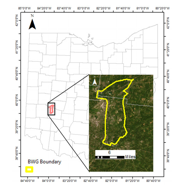
Wetlands are invaluable ecosystems, offering essential services such as carbon sequestration, water purification, flood control and habitat for countless aquatic species. However, these critical environments are under increasing threat from factors like industrialization and agricultural expansion. In this research, we focused on small-sized wetlands, typically less than 10 acres in size, due to their unique ecological roles and groundwater recharge contributions. To effectively protect and manage these wetlands, precise mapping and monitoring are essential. To achieve this, we exploited the capabilities of Sentinel-2 imagery and employ a range of machine learning algorithms, including Random Forest (RF), Classification and Regression Tree (CART), Gradient Tree Boost (GTB), Naive Bayes (NB), k-nearest neighbors (KNN) and Support Vector Machine (SVM). Our evaluation used variables, such as spectral bands, indices and image texture. We also utilized Google Earth Engine (GEE) for streamlined data processing and visualization. We found that Random Forest (RF) and Gradient Tree Boost (GTB) outperformed other classifiers according to the performance evaluation. The Normalized Difference Water Index (NDWI) came out to be one of the important predictors in mapping wetlands. By exploring the synergistic potential of these algorithms, we aim to address existing gaps and develop an optimized approach for accurate small-sized wetland mapping. Our findings will be useful in understanding the value of small wetlands and their conservation in the face of environmental challenges. They will also lay the framework for future wetland research and practical uses.

Keywords:

Citation: Eric Ariel L. Salas, Sakthi Subburayalu Kumaran, Robert Bennett, Leeoria P. Willis, Kayla Mitchell. Machine Learning-Based Classification of Small-Sized Wetlands Using Sentinel-2 Images[J]. AIMS Geosciences, 2024, 10(1): 62-79. doi: 10.3934/geosci.2024005

Related Papers:

[1]	Changdev P. Jadhav, Tanisha B. Dale, Vaijanath L. Chinchane, Asha B. Nale, Sabri T. M. Thabet, Imed Kedim, Miguel Vivas-Cortez . On solutions of fractional differential equations for the mechanical oscillations by using the Laplace transform. AIMS Mathematics, 2024, 9(11): 32629-32645. doi: 10.3934/math.20241562
[2]	Duoduo Zhao, Kai Zhou, Fengming Ye, Xin Xu . A class of time-varying differential equations for vibration research and application. AIMS Mathematics, 2024, 9(10): 28778-28791. doi: 10.3934/math.20241396
[3]	Takumi Washio, Akihiro Fujii, Toshiaki Hisada . On random force correction for large time steps in semi-implicitly discretized overdamped Langevin equations. AIMS Mathematics, 2024, 9(8): 20793-20810. doi: 10.3934/math.20241011
[4]	Omar Bazighifan, Areej A. Al-moneef, Ali Hasan Ali, Thangaraj Raja, Kamsing Nonlaopon, Taher A. Nofal . New oscillation solutions of impulsive conformable partial differential equations. AIMS Mathematics, 2022, 7(9): 16328-16348. doi: 10.3934/math.2022892
[5]	Amjid Ali, Teruya Minamoto, Rasool Shah, Kamsing Nonlaopon . A novel numerical method for solution of fractional partial differential equations involving the $\psi$ -Caputo fractional derivative. AIMS Mathematics, 2023, 8(1): 2137-2153. doi: 10.3934/math.2023110
[6]	Ahmad Qazza, Rania Saadeh, Emad Salah . Solving fractional partial differential equations via a new scheme. AIMS Mathematics, 2023, 8(3): 5318-5337. doi: 10.3934/math.2023267
[7]	Aslı Alkan, Halil Anaç . The novel numerical solutions for time-fractional Fornberg-Whitham equation by using fractional natural transform decomposition method. AIMS Mathematics, 2024, 9(9): 25333-25359. doi: 10.3934/math.20241237
[8]	Shaomin Wang, Cunji Yang, Guozhi Cha . On the variational principle and applications for a class of damped vibration systems with a small forcing term. AIMS Mathematics, 2023, 8(9): 22162-22177. doi: 10.3934/math.20231129
[9]	Armin Hadjian, Juan J. Nieto . Existence of solutions of Dirichlet problems for one dimensional fractional equations. AIMS Mathematics, 2022, 7(4): 6034-6049. doi: 10.3934/math.2022336
[10]	Paul Bosch, José M. Rodríguez, José M. Sigarreta . Oscillation results for a nonlinear fractional differential equation. AIMS Mathematics, 2023, 8(5): 12486-12505. doi: 10.3934/math.2023627

Abstract

1. Introduction

The theory of fractional calculus has played an important role in engineering and natural sciences. Currently, the concept of fractional calculus has been effectively used in many social, physical, signal, image processing, biological and engineering problems. Further, it has been realized that a fractional system provides a more accurate interpretation than the integer-order system in many real modeling problems. For more details, one can refer to ^{[1,2,3,4,5,6,7,8,9,10]}.

Oscillation phenomena take part in different models of real world applications; see for instance the papers ^{[11,12,13,14,15,16,17]} and the papers cited therein. More precisely, we refer the reader to the papers ^[18,19] on bio-mathematical models where oscillation and/or delay actions may be formulated by means of cross-diffusion terms. Recently and although it is rare, the study on the oscillation of fractional partial differential equations has attracted many researchers. In ^{[20,21,22,23]}, the researchers have established the requirements of the oscillation for certain kinds of fractional partial differential equations.

In ^[24], Luo et al. studied the oscillatory behavior of the fractional partial differential equation of the form

$\begin{align*} &D_{+, t}^{1+\alpha}u(y, t)+p( t)D_{+, t}^{\alpha}u(y, t)+q(y, t)\int_{0}^{ t}( t-\hbar)^{-\alpha}u(y, \hbar)d\hbar\\ & = a( t)\Delta u(y, t)+\sum\limits_{i = 1}^{m}a_{i}( t)\Delta u(y, t-\tau_{i}), \quad (y, t)\in Q\times \mathbb{R}_{+} = H \end{align*}$

subject to either of the following boundary conditions

$\begin{align*} \frac{\partial u(y, t)}{\partial \nu}+\beta(y, t)u(y, t)& = 0, \quad (y, t)\in \partial Q\times \mathbb{R}_{+}\, , \\ u(y, t)& = 0, \quad (y, t)\in \partial Q \times \mathbb{R}_{+}\, . \end{align*}$

They have obtained some sufficient conditions for the oscillation of all solutions of this kind of fractional partial differential equations by using the integral averaging technique and Riccati transformations.

On other hand in ^[25], Xu and Meng considered a fractional partial differential equation of the form

$\begin{align*} &D_{+, t}^{\alpha}(r( t)D_{+, t}^{\alpha}u(y, t))+p( t)D_{+, t}^{\alpha}u(y, t)+q(y, t)f(u(y, t))\\ & = a( t)\Delta u(y, t)+\sum\limits_{i = 1}^{m}b_{i}( t)\Delta u(y, t-\tau_{i}), \quad (y, t)\in Q\times \mathbb{R}_{+} = H \end{align*}$

with the Robin boundary condition

$\frac{\partial u(y, t)}{\partial N}+g(y, t)u(y, t) = 0, \quad (y, t)\in \partial Q\times \mathbb{R}_{+},$

they obtained some oscillation criteria using the integral averaging technique and Riccati transformations.

Prakash et al. ^[26] considered the oscillation of the fractional differential equation

$\begin{align*} \frac{\partial}{\partial t}(r( t)D_{+, t}^{\alpha}u(y, t))+q(y, t)f\biggl(\int_{0}^{ t}( t-v)^{-\alpha}u(y, v)dv\biggl) = a( t)\Delta u(y, t), (y, t)\in Q\times \mathbb{R}_{+} \end{align*}$

with the Neumann boundary condition

$\begin{align*} \frac{\partial u(y, t)}{\partial N} = 0, \quad (y, t)\in \partial Q\times \mathbb{R}_{+}, \end{align*}$

they obtained some oscillation criteria by using the integral averaging technique and Riccati transformations.

Furthermore in ^[27], Ma et al. considered the forced oscillation of the fractional partial differential equation with damping term of the form

$\begin{align*} \frac{\partial}{\partial t}(r( t)D_{+, t}^{\alpha}u(y, t))+p( t)D_{+, t}^{\alpha}u(y, t)+q(y, t)f(u(y, t)) = a( t)\Delta u(y, t)+\tilde{g}(y, t), \quad (y, t)\in Q\times \mathbb{R}_{+} \end{align*}$

with the boundary condition

$\frac{\partial u(y, t)}{\partial N}+\beta(y, t)u(y, t) = 0, \quad (y, t)\in \partial Q\times \mathbb{R}_{+}\, ,$

they obtained some oscillation criteria by using the integral averaging technique.

From the above mentioned literature, one can notice that the Riccati transformation method has been incorporated into the proof of the oscillation results. Unlike previous results, however, we study in this paper the forced oscillation of the fractional partial differential equation with the damping term of the form

$\begin{align} &\frac{\partial}{\partial t}\left(a( t)\frac{\partial}{\partial t}\left(r(t)g\left(D_{+, t}^{\alpha} u(y, t)\right)\right)\right)+p( t)\frac{\partial}{\partial t}\left(r( t)g(D_{+, t}^{\alpha} u(y, t))\right)\\ & = b( t)\Delta u(y, t)+\sum\limits_{i = 1}^{m} a_{i}( t)\Delta u(y, t-\tau_{i})\\ &\quad-q(y, t)\int_{0}^{ t}( t-\hbar)^{-\alpha}u(y, \hbar)d\hbar+f(y, t), \quad (y, t)\in Q \times \mathbb{R_{+}} = H \end{align}$

(1.1)

via the application of the integral averaging technique only. Equation (1.1) is presented under a high degree of generality providing a general platform for many particular cases. Here, $D^{\alpha}_{+, t}u(y, t)$ is the Riemann-Liouville fractional partial derivative of order $\alpha$ of $u, \alpha\in (0, 1),$ $\Delta$ is the Laplacian in $\mathbb{R}^{n}$ , i.e.,

$\Delta u(y, t) = \sum^{n}_{r = 1}\frac{\partial^{2}u(y, t)}{\partial y_{r}^{2}},$

$Q$ is a bounded domain of $\mathbb{R}^{n}$ with the piecewise smooth boundary $\partial Q$ and $\mathbb{R}_{+}: = (0, \infty)$ .

Further, we assume the Robin and Dirichlet boundary conditions

$\begin{equation} \frac{\partial u(y, t)}{\partial N}+\gamma (y, t)u(y, t) = 0, \quad (y, t)\in \partial Q \times \mathbb{R}_{+} \end{equation}$

(1.2)

and

$\begin{equation} u(y, t) = 0, \quad (y, t)\in \partial Q \times \mathbb{R}_{+}, \end{equation}$

(1.3)

where $N$ is the unit outward normal to $\partial Q$ and $\gamma(y, t) > 0$ is a continuous function on $\partial Q \times \mathbb{R}_{+}$ . The following conditions are assumed throughout:

$\bf (H_{1})$ $a(t)\in C^{1}([t_{0}, \infty); \mathbb{R}_{+})$ and $r(t)\in C^{2}([t_{0}, \infty); \mathbb{R}_{+})$ ;

$\bf (H_{2})$ $g(t)\in C^{2}(\mathbb{R}; \mathbb{R})$ is an increasing function and there exists a positive constant $k$ such that $\frac{y}{g(y)} = k > 0,$ $y g(y)\neq 0$ for $y\neq 0$ ;

$\bf (H_{3})$ $p(t)\in C([t_{0}, \infty); \mathbb{R})$ and $A(t) = \int_{ t_{0}}^{ t}\frac{p(\zeta)}{a(\zeta)}d\zeta$ ;

$\bf (H_{4})$ $b(t), a_{i}(t)\in C(\mathbb{R_{+}}; \mathbb{R_{+}})$ and $\tau_{i}$ are non-negative constants, $i\in I_{m} = \{1, 2, \ldots, m\}$ ;

$\bf (H_{5})$ $q(y, t)\in C(H; \mathbb{R}_{+})$ and $q(t) = \min_{ y\in Q}q(y, t)$ ;

$\bf (H_{6})$ $f(y, t)\in C(\bar{H}; \mathbb{R})$ .

By a solution of the problems (1.1) and (1.2) (or (1.1)–(1.3)), we mean a function $u(y, t)\in C^{2+\alpha}(\bar{Q}\times[0, \infty)),$ which satisfies (1.1) on $H$ and the boundary condition (1.2) (or (1.3)).

A solution $u(y, t)$ of (1.1) is said to be oscillatory if it is neither eventually positive nor eventually negative. Otherwise, it is non-oscillatory.

The rest of the paper is organized as follows. Some basic definitions and known lemmas are included in Section 2. In Sections 3 and 4, we study the oscillations of (1.1) and (1.2), and (1.1) and (1.3), respectively. Section 5 deals with some applications for the sake of showing the feasibility and effectiveness of our results. Lastly, we add a conclusion in Section 6.

2. Preliminaries

Before we start the main work, we present some basic lemmas and definitions which are applied in what follows.

Definition 1. ^[4] The Riemann-Liouville fractional integral of order $\alpha > 0$ of a function $y: \mathbb{R}_{+}\rightarrow \mathbb{R}$ on the half-axis $\mathbb{R}_{+}$ is defined by

$\begin{equation*} (I^{\alpha}_{+}y)( t): = \frac{1}{\Gamma(\alpha)}\int^{ t}_{0}( t-\vartheta)^{\alpha-1}y(\vartheta)d\vartheta, \quad t > 0 \end{equation*}$

provided the right-hand side is pointwise defined on $\mathbb{R}_{+}$ , where $\Gamma$ is the gamma function.

Definition 2. ^[4] The Riemann-Liouville fractional derivative of order $\alpha > 0$ of a function $y:\mathbb{R}_{+} \rightarrow \mathbb{R}$ on the half-axis $\mathbb{R}_{+}$ is defined by

$\begin{equation*} (D_{+}^{\alpha}y)( t): = \frac{d^{\lceil \alpha \rceil}}{d t^{\lceil \alpha \rceil}}\left(I_{+}^{\lceil \alpha \rceil -\alpha}y\right)( t), \quad t > 0 \end{equation*}$

provided the right-hand side is pointwise defined on $\mathbb{R}_{+}$ , where $\lceil \alpha \rceil$ is the ceiling function of $\alpha$ .

Definition 3. ^[4] The Riemann-Liouville fractional partial derivative of order $0 < \alpha < 1$ with respect to $t$ of a function $u(y, t)$ is defined by

$\begin{equation*} (D^{\alpha}_{+, t}u)(y, t): = \frac{1}{\Gamma(1-\alpha)}\frac{\partial}{\partial t}\int^{ t}_{0}( t-\vartheta)^{-\alpha}u(y, \vartheta)d\vartheta \end{equation*}$

provided the right-hand side is pointwise defined on $\mathbb{R}_{+}$ .

Lemma 1. ^[4] Let $y$ be a solution of (1.1) and

$\begin{equation*} L( t): = \int^{ t}_{0}( t-\vartheta)^{-\alpha}y(\vartheta)d\vartheta \end{equation*}$

for $\alpha \in (0, 1)$ and $t > 0.$ Then

$\begin{equation*} L^{\prime}( t) = \Gamma (1-\alpha)(D^{\alpha}_{+}y)( t). \end{equation*}$

Lemma 2. ^[4] Let $\alpha \ge 0, m\in\mathbb{N}$ and $D = \frac{d}{d t}$ . If the fractional derivatives $(D_{a+}^{\alpha}y)(t)$ and $(D_{a+}^{\alpha+m}y)(t)$ exist, then

$\begin{align*} \left(D^{m}D_{a+}^{\alpha}y\right)( t) = (D_{a+}^{\alpha+m}y)( t). \end{align*}$

Lemma 3. ^[4] If $\alpha\in(0, 1)$ , then

$\left(I_{a+}^{\alpha}D_{a+}^{\alpha}y\right)( t) = y( t)-\frac{y_{1-\alpha}(a)}{\Gamma(\alpha)}( t-a)^{\alpha-1},$

where $y_{1-\alpha}(t) = (I_{a+}^{1-\alpha}y)(t)$ .

Lemma 4. ^[5] The smallest eigenvalue $\beta_{0}$ of the Dirichlet problem

$\begin{align*} \Delta \omega(y)+\beta \omega(y)& = 0\mathit{\text{ in }}Q\\ \omega(y)& = 0 \mathit{\text{ on }} \partial Q \end{align*}$

is positive and the corresponding eigenfunction $\phi(y)$ is positive in $Q.$

3. Oscillation of (1.1) and (1.2)

In this section, we establish the oscillation criteria for (1.1) and (1.2).

Theorem 1. If $\bf {(H_{1})-(H_{6})}$ are valid, $\lim\limits_{ t\to\infty}I_{+}^{1-\alpha}U(0) = C_{0}$ and if

$\begin{equation} \liminf\limits_{ t\to\infty}\int_{0}^{ t}\frac{( t-\hbar)^{\alpha-1}}{r(\hbar)}\left[C_{2}+\int_{ t_{0}}^{\hbar}\frac{C_{1}}{e^{A(\tau)}a(\tau)}d\tau+\int_{ t_{0}}^{\hbar}\frac{1}{e^{A(\tau)}a(\tau)}\left(\int_{ t_{0}}^{\tau}e^{A(\zeta)}F(\zeta)d\zeta\right)d\tau \right]d\hbar < 0 \end{equation}$

(3.1)

and

$\begin{equation} \limsup\limits_{ t\to\infty}\int_{0}^{ t}\frac{( t-\hbar)^{\alpha-1}}{r(\hbar)}\left[C_{2}+\int_{ t_{0}}^{\hbar}\frac{C_{1}}{e^{A(\tau)}a(\tau)}d\tau+\int_{ t_{0}}^{\hbar}\frac{1}{e^{A(\tau)}a(\tau)}\left(\int_{ t_{0}}^{\tau}e^{A(\zeta)}F(\zeta)d\zeta\right)d\tau \right]d\hbar > 0 \end{equation}$

(3.2)

for some constants $C_{0}, C_{1}$ and $C_{2}$ with $F(t) = \int_{Q}f(y, t)dy$ , then all solutions of (1.1) and (1.2) are oscillatory.

Proof. If $u(y, t)$ is a non-oscillatory solution of (1.1) and (1.2) then there exists a $t_{0}\ge 0$ such that $u(y, t) > 0$ (or $u(y, t) < 0), t\ge t_{0}.$

Case $1$ . Let $u(y, t) > 0$ for $t\ge t_{0}.$ Integrating (1.1) over $Q,$ we get

$\begin{align} &\frac{d}{d t}\left(a( t)\frac{d}{d t}\left(r( t)g(D_{+}^{\alpha} U( t))\right)\right)+p( t)\frac{d}{d t}\left(r( t)g(D_{+}^{\alpha} U( t))\right)\\ & = b( t)\int_{Q}\Delta u(y, t)dy+\sum\limits_{i = 1}^{m} a_{i}( t)\int_{Q}\Delta u(y, t-\tau_{i})dy\\ &\quad-\int_{Q}\left(q(y, t)\int_{0}^{ t}( t-\hbar)^{-\alpha}u(y, \hbar)d\hbar\right)dy+\int_{Q}f(y, t)dy, \end{align}$

(3.3)

where $U(t) = \int_{Q}u(y, t)dy$ with $U(t) > 0.$ By (1.2) and Green's formula, we have

$\begin{equation} \int_{Q}\Delta u(y, t)dy = \int_{\partial Q}\frac{\partial u}{\partial N}d\zeta = -\int_{\partial Q} \gamma(y, t)u(y, t)d\zeta < 0 \end{equation}$

(3.4)

and

$\begin{equation} \int_{Q}\Delta u(y, t-\tau_{i})dy < 0. \end{equation}$

(3.5)

Also, by $\bf {(H_{5})},$ one can get

$\begin{align} \int_{Q}\left(q(y, t)\int_{0}^{ t}( t-\hbar)^{-\alpha}u(y, \hbar)d\hbar\right)dy&\ge q( t)\int_{0}^{ t}( t-\hbar)^{-\alpha}\left(\int_{Q}u(y, \hbar)dy\right)d\hbar\\ & = q( t)L( t), \end{align}$

(3.6)

where $L(t) = \int_{0}^{ t}(t-\hbar)^{-\alpha}U(\hbar)d\hbar.$ Because of the inequalities (3.4)–(3.6), (3.3) becomes

$\begin{align*} \frac{d}{d t}\left(a( t)\frac{d}{d t}\left(r( t)g(D_{+}^{\alpha} U( t))\right)\right)+p( t)\frac{d}{d t}\left(r( t)g(D_{+}^{\alpha} U( t))\right)\le -q( t)L( t)+F( t)\le F( t). \end{align*}$

Thus, we get

$\begin{align*} \left(e^{A( t)}a( t)\left(r( t)g(D_{+}^{\alpha}U( t))\right)^{\prime}\right)^{\prime} = e^{A( t)}\left(\left(a( t)\left(r( t)g(D_{+}^{\alpha} U( t))\right)^{\prime}\right)^{\prime}+p( t)\left(r( t)g(D_{+}^{\alpha} U( t))\right)^{\prime}\right)\nonumber \le e^{A(t)}F(t). \end{align*}$

Integrating the above inequality over $[t_{0}, t]$ , one can get

$\begin{equation*} e^{A( t)}a( t)\left(r( t)g(D_{+}^{\alpha}U( t))\right)^{\prime}\le\int_{ t_{0}}^{ t} e^{A(\zeta)}F(\zeta)d\zeta+C_{1}, \end{equation*}$

where

$C_{1} = e^{A( t_{0})}a( t_{0})\left(r( t_{0})g(D_{+}^{\alpha}U( t_{0}))\right)^{\prime}.$

Again integrating the above inequality over $[t_{0}, t]$ , we get

$\begin{equation*} r( t)g(D_{+}^{\alpha}U( t))\le C_{2}+\int_{ t_{0}}^{ t}\frac{C_{1}}{e^{A(\tau)}a(\tau)}d\tau+\int_{ t_{0}}^{ t}\frac{1}{e^{A(\tau)}a(\tau)}\left(\int_{ t_{0}}^{\tau} e^{A(\zeta)}F(\zeta)d\zeta\right)d\tau, \end{equation*}$

where $C_{2} = r(t_{0})g(D_{+}^{\alpha}U(t_{0})).$ Then using $\bf {(H_{5})}$ , we obtain

$\begin{equation*} \frac{D_{+}^{\alpha}U( t)}{k}\le \frac{C_{2}}{r( t)}+\frac{1}{r( t)}\int_{ t_{0}}^{ t}\frac{C_{1}}{e^{A(\tau)}a(\tau)}d\tau+\frac{1}{r( t)}\int_{ t_{0}}^{ t}\frac{1}{e^{A(\tau)}a(\tau)}\left(\int_{ t_{0}}^{\tau} e^{A(\zeta)}F(\zeta)d\zeta\right)d\tau. \end{equation*}$

Applying the Riemann-Liouville fractional integral operator of order $\alpha$ to the above inequality and using Lemma 3, we obtain

$\begin{align*} U( t)-\frac{I_{0}^{1-\alpha}U(0)}{\Gamma(\alpha)} t^{\alpha-1}&\le\frac{k}{\Gamma(\alpha)} \int_{0}^{ t}\frac{( t-\hbar)^{\alpha-1}}{r(\hbar)}\biggl[C_{2}+\int_{ t_{0}}^{\hbar}\frac{C_{1}}{e^{A(\tau)}a(\tau)}d\tau\\ &\quad+\int_{ t_{0}}^{\hbar}\frac{1}{e^{A(\tau)}a(\tau)}\left(\int_{ t_{0}}^{\tau} e^{A(\zeta)}F(\zeta)d\zeta\right)d\tau\biggl]d\hbar\, . \end{align*}$

Then

$\begin{align*} \liminf\limits_{ t\to\infty}U( t)&\le\liminf\limits_{ t\to\infty}\frac{C_{0}}{\Gamma(\alpha)} t^{\alpha-1}+\liminf\limits_{ t\to\infty}\left\{\frac{k}{\Gamma(\alpha)} \int_{0}^{ t}\frac{( t-\hbar)^{\alpha-1}}{r(\hbar)}\left[C_{2}+\int_{ t_{0}}^{\hbar}\frac{C_{1}}{e^{A(\tau)}a(\tau)}d\tau\right.\right.\\ &\quad\left.\left.+\int_{ t_{0}}^{\hbar}\frac{1}{e^{A(\tau)}a(\tau)}\left(\int_{ t_{0}}^{\tau} e^{A(\zeta)}F(\zeta)d\zeta\right)d\tau\right]d\hbar\right\}. \end{align*}$

Therefore, by our hypothesis, as given by (3.1), we get $\liminf_{ t\to\infty}U(t)\le 0$ . This leads to a contradiction to $U(t) > 0.$

Case $2$ . Let $u(y, t) < 0$ for $t\ge t_{0}.$ Just as in Case $1,$ we can obtain that (3.3) holds and $U(t) < 0.$ By (1.2) and Green's formula, we get

$\begin{equation} \int_{Q}\Delta u(y, t)dy = \int_{\partial Q}\frac{\partial u}{\partial N}d\zeta = -\int_{\partial Q} \gamma(y, t)u(y, t)d\zeta > 0 \end{equation}$

(3.7)

and

$\begin{equation} \int_{Q}\Delta u(y, t-\tau_{i})dy > 0. \end{equation}$

(3.8)

Also, by $\bf {(H_{5})},$ we have

$\begin{align} \int_{Q}\left(q(y, t)\int_{0}^{ t}( t-\hbar)^{-\alpha}u(y, \hbar)d\hbar\right)dy&\le q( t)\int_{0}^{ t}( t-\hbar)^{-\alpha}\left(\int_{Q}u(y, \hbar)dy\right)d\hbar\\ & = q( t)L( t). \end{align}$

(3.9)

Because of the inequalities (3.7)–(3.9), (3.3) becomes

$\begin{equation} \frac{d}{d t}\left(a( t)\frac{d}{d t}\left(r( t)g(D_{+}^{\alpha} U( t))\right)\right)+p( t)\frac{d}{d t}\left(r( t)g(D_{+}^{\alpha} U( t))\right)\ge -q( t)L( t)+F(t)\ge F(t), \end{equation}$

(3.10)

that is,

$\left(e^{A( t)}a( t)\left(r( t)g(D_{+}^{\alpha}U( t))\right)^{\prime}\right)^{\prime} =\\ e^{A( t)}\left(\left(a( t)\left(r( t)g(D_{+}^{\alpha} U( t))\right)^{\prime}\right)^{\prime}+p( t)\left(r( t)g(D_{+}^{\alpha} U( t))\right)^{\prime}\right)\nonumber \ge e^{A( t)}F( t).$

Integrating the above inequality over [ $t_{0}, t$ ], we have

$\begin{equation*} e^{A( t)}a( t)\left(r( t)g(D_{+}^{\alpha}U( t))\right)^{\prime}\ge\int_{ t_{0}}^{ t} e^{A(\zeta)}F(\zeta)d\zeta+C_{1}, \end{equation*}$

where

$C_{1} = e^{A( t_{0})}a( t_{0})\left(r( t_{0})g(D_{+}^{\alpha}U( t_{0}))\right)^{\prime}.$

Again integrating the above inequality over [ $t_{0}, t$ ], we obtain

$\begin{equation*} r( t)g(D_{+}^{\alpha}U( t))\ge C_{2}+\int_{ t_{0}}^{ t}\frac{C_{1}}{e^{A(\tau)}a(\tau)}d\tau+\int_{ t_{0}}^{ t}\frac{1}{e^{A(\tau)}a(\tau)}\left(\int_{ t_{0}}^{\tau} e^{A(\zeta)}F(\zeta)d\zeta\right)d\tau, \end{equation*}$

where $C_{2} = r(t_{0})g(D_{+}^{\alpha}U(t_{0})).$ Then using $\bf {(H_{5})}$ , we obtain

$\begin{align*} \frac{D_{+}^{\alpha}U( t)}{k}\ge \frac{C_{2}}{r( t)}+\frac{1}{r( t)}\int_{ t_{0}}^{ t}\frac{C_{1}}{e^{A(\tau)}a(\tau)}d\tau+\frac{1}{r( t)}\int_{ t_{0}}^{ t}\frac{1}{e^{A(\tau)}a(\tau)}\biggl(\int_{ t_{0}}^{\tau} e^{A(\zeta)}F(\zeta)d\zeta\biggl)d\tau. \end{align*}$

Applying the Riemann-Liouville fractional integral operator of order $\alpha$ to the above inequality and using Lemma $3,$ we obtain

$\begin{align*} U( t)-\frac{I_{0}^{1-\alpha}U(0)}{\Gamma(\alpha)} t^{\alpha-1}\ge&\frac{k}{\Gamma(\alpha)} \int_{0}^{ t}\frac{( t-\hbar)^{\alpha-1}}{r(\hbar)}\biggl[C_{2}+\int_{ t_{0}}^{\hbar}\frac{C_{1}}{e^{A(\tau)}a(\tau)}d\tau\\&+\int_{ t_{0}}^{\hbar}\frac{1}{e^{A(\tau)}a(\tau)}\biggl(\int_{ t_{0}}^{\tau} e^{A(\zeta)}F(\zeta)d\zeta\biggl)d\tau\biggl]d\hbar. \end{align*}$

Then

$\begin{align*} \limsup\limits_{ t\to\infty}U( t)&\ge\limsup\limits_{ t\to\infty}\frac{C_{0}}{\Gamma(\alpha)} t^{\alpha-1}+\limsup\limits_{ t\to\infty}\biggl\{\frac{k}{\Gamma(\alpha)} \int_{0}^{ t}\frac{( t-\hbar)^{\alpha-1}}{r(\hbar)}\biggl[C_{2}+\int_{ t_{0}}^{\hbar}\frac{C_{1}}{e^{A(\tau)}a(\tau)}d\tau\\ &\quad+\int_{ t_{0}}^{\hbar}\frac{1}{e^{A(\tau)}a(\tau)}\biggl(\int_{ t_{0}}^{\tau} e^{A(\zeta)}F(\zeta)d\zeta\biggl)d\tau\biggl]d\hbar\biggl\}. \end{align*}$

Therefore, by our hypothesis given by (3.2), we get $\limsup_{ t\to\infty}U(t)\ge 0$ . This leads to a contradiction to $U(t) < 0.$

4. Oscillation of (1.1) and (1.3)

In this section, we establish the oscillation criteria for (1.1) and (1.3).

Theorem 2. If $\bf {(H_{1})-(H_{5})}$ are valid, $\lim\limits_{ t\to\infty}I_{+}^{1-\alpha}U_{1}(0) = A_{1}$ and if

$\begin{equation} \liminf\limits_{ t\to\infty}\int_{0}^{ t}\frac{( t-\hbar)^{\alpha-1}}{r(\hbar)}\biggl[C_{2}+\int_{ t_{0}}^{\hbar}\frac{C_{1}}{e^{A(\tau)}a(\tau)}d\tau+\int_{ t_{0}}^{\hbar}\frac{1}{e^{A(\tau)}a(\tau)}\biggl(\int_{ t_{0}}^{\tau}e^{A(\zeta)}F_{1}(\zeta)d\zeta\biggl)d\tau \biggl]d\hbar < 0 \end{equation}$

(4.1)

and

$\begin{equation} \limsup\limits_{ t\to\infty}\int_{0}^{ t}\frac{( t-\hbar)^{\alpha-1}}{r(\hbar)}\biggl[C_{2}+\int_{ t_{0}}^{\hbar}\frac{C_{1}}{e^{A(\tau)}a(\tau)}d\tau+\int_{ t_{0}}^{\hbar}\frac{1}{e^{A(\tau)}a(\tau)}\biggl(\int_{ t_{0}}^{\tau}e^{A(\zeta)}F_{1}(\zeta)d\zeta\biggl)d\tau \biggl]d\hbar > 0 \end{equation}$

(4.2)

for some constants $A_{1}, C_{1}$ and $C_{2}$ with

$F_{1}( t) = \int_{Q}f(y, t)\phi(y)dy\;\mathit{\text{and}}\; U_{1}( t) = \int_{Q}u(y, t)\phi(y)dy,$

then all solutions of $(1.1)$ and $(1.3)$ are oscillatory.

Proof. If $u(y, t)$ is a non-oscillatory solution of (1.1) and (1.3) then there exists a $t_{0}\ge 0$ such that $u(y, t) > 0$ (or $u(y, t) < 0$ ) for $t\ge t_{0}.$

Case $1$ . Let $u(y, t) > 0$ for $t\ge t_{0}.$ Multiplying $(1.1)$ by $\phi(y)$ and then integrating over $Q,$ we get

$\begin{align} &\int_{Q}\frac{\partial}{\partial t}\left(a( t)\frac{\partial}{\partial t}\left(r( t)g(D_{+, t}^{\alpha} u(y, t))\right)\right)\phi(y)dy+\int_{Q}p( t)\frac{\partial}{\partial t}\left(r( t)g(D_{+, t}^{\alpha} u(y, t))\right)\phi(y)dy\\ & = \int_{Q}b( t)\Delta u(y, t)\phi(y)dy+\int_{Q}\sum\limits_{i = 1}^{m} a_{i}( t)\Delta u(y, t-\tau_{i})\phi(y)dy\\ &\quad-\int_{Q}\left(q(y, t)\int_{0}^{ t}( t-\hbar)^{-\alpha}u(y, \hbar)d\hbar\right)\phi(y)dy+\int_{Q}f(y, t)\phi(y)dy. \end{align}$

(4.3)

By Lemma 4 and Green's formula, we have

$\begin{equation} \int_{Q}\Delta u(y, t)\phi(y)dy = \int_{Q}u(y, t)\Delta \phi(y)dy = -\beta_{0}\int_{Q}u(y, t)\phi(y)dy < 0 \end{equation}$

(4.4)

and

$\begin{equation} \int_{Q}\Delta u(y, t-\tau_{i})\phi(y)dy < 0. \end{equation}$

(4.5)

Also, by $\bf {(H_{5})},$ we get

$\begin{align} \int_{Q}\left(q(y, t)\int_{0}^{ t}( t-\hbar)^{-\alpha}u(y, \hbar)\phi(y)d\hbar\right)dy&\ge q( t)\int_{0}^{ t}( t-\hbar)^{-\alpha}\left(\int_{Q}u(y, \hbar)\phi(y)dy\right)d\hbar\\ & = q( t)L_{1}( t), \end{align}$

(4.6)

where

$L_{1}( t) = \int_{0}^{ t}( t-\hbar)^{-\alpha}U_{1}(\hbar)d\hbar > 0.$

Because of the inequalities (4.4)–(4.6), (4.3) becomes

$\begin{equation*} \frac{d}{d t}\left(a( t)\frac{d}{d t}\left(r( t)g(D_{+}^{\alpha} U_{1}( t))\right)\right)+p( t)\frac{d}{d t}\left(r( t)g(D_{+}^{\alpha} U_{1}( t))\right)\le -q( t)L_{1}( t)+F_{1}( t)\le F_{1}( t), \end{equation*}$

that is,

$\left(e^{A( t)}a( t)\left(r( t)g(D_{+}^{\alpha}U_{1}( t))\right)^{\prime}\right)^{\prime} = \\ e^{A( t)}\biggl[\biggl(a( t)\biggl(r( t)g(D_{+}^{\alpha} U_{1}( t))\biggl)^{\prime}\biggl)^{\prime}+p( t)\biggl(r( t)g(D_{+}^{\alpha} U_{1}( t))\biggl)^{\prime}\biggl]\le e^{A( t)}F_{1}( t).$

Integrating the above inequality over $[t_{0}, t]$ , we have

$\begin{equation*} e^{A( t)}a( t)\left(r( t)g(D_{+}^{\alpha}U_{1}( t))\right)^{\prime}\le\int_{ t_{0}}^{ t} e^{A(\zeta)}F_{1}(\zeta)d\zeta+C_{1}, \end{equation*}$

where

$C_{1} = e^{A( t_{0})}a( t_{0})\left(r( t_{0})g(D_{+}^{\alpha}U_{1}( t_{0}))\right)^{\prime}.$

Again integrating the above inequality over $[t_{0}, t]$ , we have

$\begin{equation*} r( t)g(D_{+}^{\alpha}U_{1}( t))\le C_{2}+\int_{ t_{0}}^{ t}\frac{C_{1}}{e^{A(\tau)}a(\tau)}d\tau+\int_{ t_{0}}^{ t}\frac{1}{e^{A(\tau)}a(\tau)}\left(\int_{ t_{0}}^{\tau} e^{A(\zeta)}F_{1}(\zeta)d\zeta\right)d\tau, \end{equation*}$

where $C_{2} = r(t_{0})g(D_{+}^{\alpha}U_{1}(t_{0})).$ Then using $\bf {(H_{5})}$ , we obtain

$\begin{equation*} \frac{D_{+}^{\alpha}U_{1}( t)}{k}\le \frac{C_{2}}{r( t)}+\frac{1}{r( t)}\int_{ t_{0}}^{ t}\frac{C_{1}}{e^{A(\tau)}a(\tau)}d\tau+\frac{1}{r( t)}\int_{ t_{0}}^{ t}\frac{1}{e^{A(\tau)}a(\tau)}\left(\int_{ t_{0}}^{\tau} e^{A(\zeta)}F_{1}(\zeta)d\zeta\right)d\tau. \end{equation*}$

Applying the Riemann-Liouville fractional integral operator of order $\alpha$ to the above inequality and using Lemma 3, we obtain

$\begin{align*} U_{1}( t)-\frac{I_{0}^{1-\alpha}U_{1}(0)}{\Gamma(\alpha)} t^{\alpha-1}&\le\frac{k}{\Gamma(\alpha)} \int_{0}^{ t}\frac{( t-\hbar)^{\alpha-1}}{r(\hbar)}\biggl[C_{2}+\int_{ t_{0}}^{\hbar}\frac{C_{1}}{e^{A(\tau)}a(\tau)}d\tau\\ &\quad+\int_{ t_{0}}^{\hbar}\frac{1}{e^{A(\tau)}a(\tau)}\biggl(\int_{ t_{0}}^{\tau} e^{A(\zeta)}F_{1}(\zeta)d\zeta\biggl)d\tau\biggl]d\hbar. \end{align*}$

Then

$\begin{align*} \liminf\limits_{ t\to\infty}U_{1}( t)&\le\liminf\limits_{ t\to\infty}\frac{A_{1}}{\Gamma(\alpha)} t^{\alpha-1}+\liminf\limits_{ t\to\infty}\biggl\{\frac{k}{\Gamma(\alpha)} \int_{0}^{ t}\frac{( t-\hbar)^{\alpha-1}}{r(\hbar)}\biggl[C_{2}+\int_{ t_{0}}^{\hbar}\frac{C_{1}}{e^{A(\tau)}a(\tau)}d\tau\\&+\int_{ t_{0}}^{\hbar}\frac{1}{e^{A(\tau)}a(\tau)}\biggl(\int_{ t_{0}}^{\tau} e^{A(\zeta)}F_{1}(\zeta)d\zeta\biggl)d\tau\biggl]d\hbar\biggl\}. \end{align*}$

Therefore, by our hypothesis given by (4.1), we get $\liminf_{ t\to\infty}U_{1}(t)\le 0$ . This leads to a contradiction to $U_{1}(t) > 0.$

Case $2$ . Let $u(y, t) < 0$ for $t\ge t_{0}.$ Multiplying $(1.1)$ by $\phi(y)$ and then integrating over $Q,$ one can get (4.3). Using Green's formula, we have

$\begin{equation} \int_{Q}\Delta u(y, t)\phi(y)dy = \int_{Q}u(y, t)\Delta \phi(y)dy = -\beta_{0}\int_{Q}u(y, t)\phi(y) dy > 0 \end{equation}$

(4.7)

and

$\begin{equation} \int_{Q}\Delta u(y, t-\tau_{i})\phi(y)dy > 0. \end{equation}$

(4.8)

Also, by $\bf {(H_{5})},$ we have

$\begin{align} \int_{Q}\biggl(q(y, t)\int_{0}^{ t}( t-\hbar)^{-\alpha}u(y, \hbar)d\hbar\biggl)\phi(y)dy&\le q( t)\int_{0}^{ t}( t-\hbar)^{-\alpha}\biggl(\int_{Q}u(y, \hbar)\phi(y)dy\biggl)d\hbar\\ & = q( t)L_{1}( t), \end{align}$

(4.9)

where

$L_{1}( t) = \int_{0}^{ t}( t-\hbar)^{-\alpha}U_{1}(\hbar)d\hbar < 0.$

Because of the inequalities (4.7)–(4.9), (4.3) becomes

$\begin{equation} \frac{d}{d t}\biggl(a( t)\frac{d}{d t}\biggl(r( t)g(D_{+}^{\alpha} U_{1}( t))\biggl)\biggl)+p( t)\frac{d}{d t}\biggl(r( t)g(D_{+}^{\alpha} U_{1}( t))\biggl)\ge -q( t)L_{1}( t)+F_{1}( t)\ge F_{1}( t), \end{equation}$

(4.10)

that is,

$\biggl(e^{A( t)}a( t)\biggl(r( t)g(D_{+}^{\alpha}U_{1}( t))\biggl)^{\prime}\biggl)^{\prime} = \\ e^{A( t)}\biggl(\biggl(a( t)\biggl(r( t)g(D_{+}^{\alpha} U_{1}( t))\biggl)^{\prime}\biggl)^{\prime}+p( t)\biggl(r( t)g(D_{+}^{\alpha} U_{1}( t))\biggl)^{\prime}\biggl) \ge e^{A( t)}F_{1}( t).$

Integrating the above inequality over $[t_{0}, t]$ , we get

$\begin{equation*} e^{A( t)}a( t)\left(r( t)g(D_{+}^{\alpha}U_{1}( t))\right)^{\prime}\ge\int_{ t_{0}}^{ t} e^{A(\zeta)}F_{1}(\zeta)d\zeta+C_{1}, \end{equation*}$

where

$C_{1} = e^{A( t_{0})}a( t_{0})\left(r( t_{0})g(D_{+}^{\alpha}U_{1}( t_{0}))\right)^{\prime}.$

Again integrating the above inequality over $[t_{0}, t]$ , we get

$\begin{equation*} r( t)g(D_{+}^{\alpha}U_{1}( t))\ge C_{2}+\int_{ t_{0}}^{ t}\frac{C_{1}}{e^{A(\tau)}a(\tau)}d\tau+\int_{ t_{0}}^{ t}\frac{1}{e^{A(\tau)}a(\tau)}\biggl(\int_{ t_{0}}^{\tau} e^{A(\zeta)}F_{1}(\zeta)d\zeta\biggl)d\tau, \end{equation*}$

where $C_{2} = r(t_{0})g(D_{+}^{\alpha}U_{1}(t_{0})).$ Then using $\bf {(H_{5})}$ , we obtain

$\begin{equation*} \frac{D_{+}^{\alpha}U_{1}( t)}{k}\ge \frac{C_{2}}{r( t)}+\frac{1}{r( t)}\int_{ t_{0}}^{ t}\frac{C_{1}}{e^{A(\tau)}a(\tau)}d\tau+\frac{1}{r( t)}\int_{ t_{0}}^{ t}\frac{1}{e^{A(\tau)}a(\tau)}\biggl(\int_{ t_{0}}^{\tau} e^{A(\zeta)}F_{1}(\zeta)d\zeta\biggl)d\tau. \end{equation*}$

Applying the Riemann-Liouville fractional integral operator of order $\alpha$ to the above inequality and using Lemma 3, we obtain

$\begin{align*} U_{1}( t)-\frac{I_{0}^{1-\alpha}U_{1}(0)}{\Gamma(\alpha)} t^{\alpha-1}&\ge\frac{k}{\Gamma(\alpha)} \int_{0}^{ t}\frac{( t-\hbar)^{\alpha-1}}{r(\hbar)}\left[C_{2}+\int_{ t_{0}}^{\hbar}\frac{C_{1}}{e^{A(\tau)}a(\tau)}d\tau\right.\\ &\quad\left.+\int_{ t_{0}}^{\hbar}\frac{1}{e^{A(\tau)}a(\tau)}\left(\int_{ t_{0}}^{\tau} e^{A(\zeta)}F_{1}(\zeta)d\zeta\right)d\tau\right]d\hbar. \end{align*}$

Then

$\begin{align*} \limsup\limits_{ t\to\infty}U_{1}( t)&\ge\limsup\limits_{ t\to\infty}\frac{A_{1}}{\Gamma(\alpha)} t^{\alpha-1}+\limsup\limits_{ t\to\infty}\left\{\frac{k}{\Gamma(\alpha)} \int_{0}^{ t}\frac{( t-\hbar)^{\alpha-1}}{r(\hbar)}\left[C_{2}+\int_{ t_{0}}^{\hbar}\frac{C_{1}}{e^{A(\tau)}a(\tau)}d\tau\right.\right.\\ &\quad\left.\left.+\int_{ t_{0}}^{\hbar}\frac{1}{e^{A(\tau)}a(\tau)}\left(\int_{ t_{0}}^{\tau} e^{A(\zeta)}F_{1}(\zeta)d\zeta\right)d\tau\right]d\hbar\right\}. \end{align*}$

Therefore, by our hypothesis given by $(4.2)$ , we get $\limsup_{ t\to\infty}U_{1}(t)\ge 0$ . This leads to a contradiction to $U_{1}(t) < 0.$

5. Applications

In this section, we give two examples to illustrate our main results.

Example 1. Let us consider the fractional partial differential system

$\begin{align} D_{+, t}^{\frac{5}{2}}u(y, t)& = \frac{1}{\pi}\Delta u(y, t)+2 t\Delta u(y, t-1)\\ &\quad-\left(y^{2}+\frac{1}{ t^{2}}\right)\int_{0}^{ t}( t-\hbar)^{-\frac{1}{2}}u(y, \hbar)d\hbar+e^{2 t}\cos (t)\sin (y), \quad (y, t)\in (0, \pi)\times \mathbb{R_{+}} \end{align}$

(5.1)

with the condition

$\begin{align} u_{y}(0, t) = u_{y}(\pi, t) = 0. \end{align}$

(5.2)

In the above, $a(t) = 1, r(t) = 1, g(t) = t, \alpha = 1/2, p(t) = 0, b(t) = 1/\pi, m = 1, a_{1}(t) = 2 t, \tau_{1} = 1$ , $q(y, t) = (y^{2}+\frac{1}{ t^{2}}), f(y, t) = e^{2 t}\cos (t) \sin (y), Q = (0, \pi), q(t) = \min_{y\in(0, \pi)}q(y, t) = 1/ t^{2}$ and $t_{0} = 0$ .

Since $F(t) = \int_{0}^{\pi}e^{2 t}\cos (t) \sin (y) dy = 2e^{2 t}\cos (t)$ and $A(t) = 0,$ we have

$\begin{align*} &\int_{0}^{ t}\frac{( t-\hbar)^{\alpha-1}}{r(\hbar)}\left[C_{2}+\int_{ t_{0}}^{\hbar}\frac{C_{1}}{e^{A(\tau)}a(\tau)}d\tau+\int_{ t_{0}}^{\hbar}\frac{1}{e^{A(\tau)}a(\tau)}\left(\int_{ t_{0}}^{\tau}e^{A(\zeta)}F(\zeta)d\zeta\right)d\tau \right]d\hbar\\ & = C_{2}\int_{0}^{ t}( t-\hbar)^{-1/2}d\hbar+C_{1}\int_{0}^{ t}( t-\hbar)^{-1/2}\left(\int_{0}^{\hbar}d\tau\right)d\hbar\\ &\quad+\frac{2}{5}\int_{0}^{ t}( t-\hbar)^{-1/2}\left(2\int_{0}^{\hbar}e^{2\tau}\cos (\tau )d\tau+\int_{0}^{\hbar}e^{2\tau}\sin (\tau) d\tau-2\int_{0}^{\hbar}d\tau\right)d\hbar\\ & = (C_{2}-6/25)\int_{0}^{ t}( t-\hbar)^{-1/2}d\hbar+(C_{1}-4/5)\int_{0}^{ t}\hbar( t-\hbar)^{-1/2}d\hbar\\ &\quad+6/25\int_{0}^{ t}e^{2\hbar}( t-\hbar)^{-1/2}\cos (\hbar) d\hbar+8/25\int_{0}^{ t}e^{2\hbar}( t-\hbar)^{-1/2}\sin( \hbar) d\hbar. \end{align*}$

Fixing $y^{2} = t-\hbar$ , then

$\begin{align} &\int_{0}^{ t}\frac{( t-\hbar)^{\alpha-1}}{r(\hbar)}\left[C_{2}+\int_{ t_{0}}^{\hbar}\frac{C_{1}}{e^{A(\tau)}a(\tau)}d\tau+\int_{ t_{0}}^{\hbar}\frac{1}{e^{A(\tau)}a(\tau)}\left(\int_{ t_{0}}^{\tau}e^{A(\zeta)}F(\zeta)d\zeta\right)d\tau \right]d\hbar\\ & = 2(C_{2}-6/25)\sqrt{ t}+4/3(C_{1}-4/5) t^{3/2}\\ &\quad+4/25e^{2 t}\left(3\cos (t) \int_{0}^{\sqrt{ t}}e^{-2y^{2}}\cos (y^{2})dy+3\sin (t)\int_{0}^{\sqrt{ t}}e^{-2y^{2}}\sin (y^{2})dy\right.\\ &\quad\left.+4\sin (t)\int_{0}^{\sqrt{ t}}e^{-2y^{2}}\cos (y^{2})dy-4\cos (t) \int_{0}^{\sqrt{ t}}e^{-2y^{2}}\sin (y^{2})dy\right). \end{align}$

(5.3)

Pointing out that

$\begin{align*} |e^{-2y^{2}}\cos (y^{2})|\le e^{-2y^{2}}, \; |e^{-2y^{2}}\sin (y^{2})|\le e^{-2y^{2}}\;\text{ and }\;\lim\limits_{ t\to\infty}\int_{0}^{\sqrt{ t}}e^{-2y^{2}}dy = \frac{\sqrt{2\pi}}{4}, \end{align*}$

we can conclude that

$\begin{align*} \lim\limits_{ t\to\infty}\int_{0}^{\sqrt{ t}}e^{-2y^{2}}\cos (y^{2})dy\quad\text{ and }\quad\lim\limits_{ t\to\infty}\int_{0}^{\sqrt{ t}}e^{-2y^{2}}\sin (y^{2})dy \end{align*}$

are convergent. Thus, we have that

$\begin{align*} &\lim\limits_{t\to\infty}\left[\cos (t) \left(3\int_{0}^{\sqrt{ t}}e^{-2y^{2}}\cos (y^{2})dy-4\int_{0}^{\sqrt{ t}}e^{-2y^{2}}\sin (y^{2})dy\right)\right.\\ &\quad\left.+\sin t\left(3\int_{0}^{\sqrt{ t}}e^{-2y^{2}}\sin (y^{2})dy+4\int_{0}^{\sqrt{ t}}e^{-2y^{2}}\cos (y^{2})dy\right)\right] \end{align*}$

is convergent. Fixing

$\begin{align*} \lim\limits_{ t\to\infty}\int_{0}^{\sqrt{ t}}e^{-2y^{2}}\cos (y^{2})dy = P, \quad\lim\limits_{ t\to\infty}\int_{0}^{\sqrt{ t}}e^{-2y^{2}}\sin (y^{2})dy = Q \end{align*}$

and considering the sequence

$\begin{align*} t_{n} = \frac{3\pi}{2}+2n\pi-\arctan \left(\frac{3P-4Q}{3Q+4P}\right), \end{align*}$

we get

$\begin{align*} &\lim\limits_{n\to\infty}\left\{\cos (t_{n}) \left(3\int_{0}^{\sqrt{ t_{n}}}e^{-2y^{2}}\cos (y^{2})dy-4\int_{0}^{\sqrt{ t_{n}}}e^{-2y^{2}}\sin (y^{2})dy\right)\right.\\ &\quad\left.+\sin (t_{n})\left(3\int_{0}^{\sqrt{ t_{n}}}e^{-2y^{2}}\sin (y^{2})dy+4\int_{0}^{\sqrt{ t_{n}}}e^{-2y^{2}}\cos (y^{2})dy\right)\right\}\\ & = \sqrt{(3P-4Q)^{2}+(3Q+4P)^{2}}\sin\left(\frac{3\pi}{2}+2n\pi-\arctan \left(\frac{3P-4Q}{3Q+4P}\right)+\arctan \left(\frac{3P-4Q}{3Q+4P}\right)\right)\\ & = 5\sqrt{P^{2}+Q^{2}}\sin\left(\frac{3\pi}{2}+2n\pi\right)\\ & = -5\sqrt{P^{2}+Q^{2}}. \end{align*}$

Since $\lim\limits_{n\to\infty} t_{n} = \infty$ , from (5.3), we have

$\begin{align*} &\liminf\limits_{ t\to\infty}\int_{0}^{ t}\frac{( t-\hbar)^{\alpha-1}}{r(\hbar)}\left[C_{2}+\int_{ t_{0}}^{\hbar}\frac{C_{1}}{e^{A(\tau)}a(\tau)}d\tau+\int_{ t_{0}}^{\hbar}\frac{1}{e^{A(\tau)}a(\tau)}\left(\int_{ t_{0}}^{\tau}e^{A(\zeta)}F(\zeta)d\zeta\right)d\tau \right]d\hbar\\ & = \liminf\limits_{n\to\infty}\left\{2(C_{2}-6/25)\sqrt{ t_{n}}+4/3(e^{-1}C_{1}-4/5) t_{n}^{3/2}+4/25e^{2 t_{n}}\left[\cos (t_{n}) \left(3\int_{0}^{\sqrt{ t_{n}}}e^{-2y^{2}}\cos (y^{2})dy\right.\right.\right.\\ &\quad\left.\left.\left.-4\int_{0}^{\sqrt{ t_{n}}}e^{-2y^{2}}\sin (y^{2})dy\right)+\sin (t_{n})\left(3\int_{0}^{\sqrt{ t_{n}}}e^{-2y^{2}}\sin (y^{2})dy+4\int_{0}^{\sqrt{ t_{n}}}e^{-2y^{2}}\cos (y^{2})dy \right)\right]\right\}\\ & = -\infty < 0. \end{align*}$

Similarly, fixing

$\begin{align*} t_{n} = \frac{\pi}{2}+2n\pi-\arctan \left(\frac{3P-4Q}{3Q+4P}\right), \end{align*}$

we get

$\begin{align*} &\lim\limits_{n\to\infty}\left[\cos (t_{n}) \left(3\int_{0}^{\sqrt{ t_{n}}}e^{-2y^{2}}\cos (y^{2})dy-4\int_{0}^{\sqrt{ t_{n}}}e^{-2y^{2}}\sin (y^{2})dy\right)\right.\\ &\quad\left.+\sin (t_{n})\left(3\int_{0}^{\sqrt{ t_{n}}}e^{-2y^{2}}\sin (y^{2})dy+4\int_{0}^{\sqrt{ t_{n}}}e^{-2y^{2}}\cos (y^{2})dy\right)\right]\\ & = 5\sqrt{P^{2}+Q^{2}}. \end{align*}$

Thus, from (5.3), we can get

$\limsup\limits_{ t\to\infty}\int_{0}^{ t}\frac{( t-\hbar)^{\alpha-1}}{r(\hbar)}\left[C_{2}+\int_{ t_{0}}^{\hbar}\frac{C_{1}}{e^{A(\tau)}a(\tau)}d\tau+\int_{ t_{0}}^{\hbar}\frac{1}{e^{A(\tau)}a(\tau)}\left(\int_{ t_{0}}^{\tau}e^{A(\zeta)}F(\zeta)d\zeta\right)d\tau \right]d\hbar\\ = \limsup\limits_{n\to\infty}\\ \left\{2(C_{2}-6/25)\sqrt{ t_{n}}+4/3(e^{-1}C_{1}-4/5) t_{n}^{3/2}+4/25e^{2 t_{n}}\left[\cos (t_{n}) \left(3\int_{0}^{\sqrt{ t_{n}}}e^{-2y^{2}}\cos (y^{2})dy\right.\right.\right.\\ \quad\left.\left.\left.-4\int_{0}^{\sqrt{ t_{n}}}e^{-2y^{2}}\sin (y^{2})dy\right)+\sin (t_{n})\left(3\int_{0}^{\sqrt{ t_{n}}}e^{-2y^{2}}\sin (y^{2})dy+4\int_{0}^{\sqrt{ t_{n}}}e^{-2y^{2}}\cos (y^{2})dy\right) \right]\right\}\\ = \infty > 0.$

Therefore, by referring to Theorem 1, the solutions of (5.1) and (5.2) are oscillatory.

Example 2. Let us consider the fractional partial differential system

$\frac{1}{1875\sqrt{\pi}}D_{+, t}^{\frac{5}{2}}u(y, t) = \frac{1}{10^{5} t^{\frac{5}{2}}}\Delta u(y, t)+\\ \left(\frac{16}{75\times 10^{2}\pi t^{3}}-\frac{16e^{2 t}\cos (t)}{5\pi t^{3}}\right)\int_{0}^{ t}( t-\hbar)^{-\frac{1}{2}}u(y, \hbar)d\hbar\\ +e^{2 t}\cos (t)\cos(10y), \quad (y, t)\in (0, \pi)\times (0, 1.5)$

(5.4)

with the condition

$\begin{align} u(0, t) = u(\pi, t) = 0. \end{align}$

(5.5)

In the above, $a(t) = 1$ , $r(t) = \frac{1}{1875\sqrt{\pi}}$ , $g(t) = t$ , $\alpha = 1/2$ , $p(t) = 0$ , $b(t) = \frac{1}{2\times 10^{5} t^{\frac{5}{2}}}$ , $m = 1$ , $a_{1}(t) = \frac{1}{2\times 10^{5} t^{\frac{5}{2}}}$ , $\tau_{1} = 0$ , $q(y, t) =$ $\frac{-16}{75\times 10^{2}\pi t^{3}}+\frac{16e^{2 t}\cos (t)}{5\pi t^{3}}, f(y, t) =$ $e^{2 t}\cos (t) \sin (y), Q = (0, \pi), q(t) = \min_{y\in(0, \pi)}q(y, t) =$ $\frac{-16}{75\times 10^{2}\pi t^{3}}+\frac{16e^{2 t}\cos (t)}{5\pi t^{3}}$ and $t_{0} = 0$ . It is obvious that $\beta_{0} = 1$ and $\phi(y) = \sin (y).$ Since $F_{1}(t) = \int_{0}^{\pi}e^{2 t}\cos (t) \cos(10y) \sin (y) dy =$ $\frac{-2}{99}e^{2 t}\cos (t)$ and $A(t) = 0,$ we have

$\begin{align*} &\int_{0}^{ t}\frac{( t-\hbar)^{\alpha-1}}{r(\hbar)}\left(C_{2}+\int_{ t_{0}}^{\hbar}\frac{C_{1}}{e^{A(\tau)}a(\tau)}d\tau+\int_{ t_{0}}^{\hbar}\frac{1}{e^{A(\tau)}a(\tau)}\left(\int_{ t_{0}}^{\tau}e^{A(\zeta)}F(\zeta)d\zeta\right)d\tau \right)d\hbar\\ & = -\frac{3750\sqrt{\pi}}{99}\int_{0}^{ t}( t-\hbar)^{\alpha-1}\left(\int_{ t_{0}}^{\hbar}\left(\int_{ t_{0}}^{\tau}e^{2\zeta}\cos (\zeta) d\zeta\right)d\tau \right)d\hbar\\ & = \frac{50\sqrt{\pi}}{11}\int_{0}^{ t}( t-\hbar)^{-1/2}d\hbar+\frac{500\sqrt{\pi}}{33}\int_{0}^{ t}\hbar( t-\hbar)^{-1/2}d\hbar\\ &\quad-\frac{50\sqrt{\pi}}{33}\left[3\int_{0}^{ t}e^{2\hbar}( t-\hbar)^{-1/2}\cos (\hbar) d\hbar+4\int_{0}^{ t}e^{2\hbar}( t-\hbar)^{-1/2}\sin( \hbar) d\hbar\right]. \end{align*}$

Fixing $y^{2} = t-\hbar$ , then

$\int_{0}^{ t}\frac{( t-\hbar)^{\alpha-1}}{r(\hbar)}\left[C_{2}+\int_{ t_{0}}^{\hbar}\frac{C_{1}}{e^{A(\tau)}a(\tau)}d\tau+\int_{ t_{0}}^{\hbar}\frac{1}{e^{A(\tau)}a(\tau)}\left(\int_{ t_{0}}^{\tau}e^{A(\zeta)}F(\zeta)d\zeta\right)d\tau \right]d\hbar\\ = \frac{10^{2}\sqrt{\pi t}}{11}+\frac{2\times 10^{3}}{99} t^{3/2}-\frac{10^{2}\sqrt{\pi}}{33}e^{2 t}\left\{3\cos (t) \int_{0}^{\sqrt{ t}}e^{-2y^{2}}\cos (y^{2})dy\right.\\ \left.+3\sin (t)\int_{0}^{\sqrt{ t}}e^{-2y^{2}}\sin (y^{2})dy+4\sin (t)\\ \int_{0}^{\sqrt{ t}}e^{-2y^{2}}\cos (y^{2})dy-4\cos (t) \int_{0}^{\sqrt{ t}}e^{-2y^{2}}\sin (y^{2})dy\right\}.$

(5.6)

Pointing out that

$|e^{-2y^{2}}\cos (y^{2})|\le e^{-2y^{2}}, \; |e^{-2y^{2}}\sin (y^{2})|\le e^{-2y^{2}}\;\text{ and }\; \lim\limits_{ t\to\infty}\int_{0}^{\sqrt{ t}}e^{-2y^{2}}dy = \frac{\sqrt{2\pi}}{4},$

we can conclude that

$\lim\limits_{ t\to\infty}\int_{0}^{\sqrt{ t}}e^{-2y^{2}}\cos (y^{2})dy\quad\text{ and }\quad\lim\limits_{ t\to\infty}\int_{0}^{\sqrt{ t}}e^{-2y^{2}}\sin (y^{2})dy$

are convergent. Thus, we have that

$\begin{align*} \lim\limits_{ t\to\infty}&\left[\cos (t) \left(3\int_{0}^{\sqrt{ t}}e^{-2y^{2}}\cos (y^{2})dy-4\int_{0}^{\sqrt{ t}}e^{-2y^{2}}\sin (y^{2})dy\right)\right.\\ &\quad\left.+\sin t\left(3\int_{0}^{\sqrt{ t}}e^{-2y^{2}}\sin (y^{2})dy+4\int_{0}^{\sqrt{ t}}e^{-2y^{2}}\cos (y^{2})dy\right)\right] \end{align*}$

is convergent. Fixing

$\lim\limits_{ t\to\infty}\int_{0}^{\sqrt{ t}}e^{-2y^{2}}\cos (y^{2})dy = P\;\text{ and }\;\lim\limits_{ t\to\infty}\int_{0}^{\sqrt{ t}}e^{-2y^{2}}\sin (y^{2})dy = Q$

and considering the sequence

$t_{n} = \frac{3\pi}{2}+2n\pi-\arctan \biggl(\frac{3P-4Q}{3Q+4P}\biggl),$

we get

$\begin{align*} \lim\limits_{n\to\infty}&\left\{\cos (t_{n}) \left(3\int_{0}^{\sqrt{ t_{n}}}e^{-2y^{2}}\cos (y^{2})dy-4\int_{0}^{\sqrt{ t_{n}}}e^{-2y^{2}}\sin (y^{2})dy\right)\right.\\ &\quad\left.+\sin (t_{n})\left(3\int_{0}^{\sqrt{ t_{n}}}e^{-2y^{2}}\sin (y^{2})dy+4\int_{0}^{\sqrt{ t_{n}}}e^{-2y^{2}}\cos (y^{2})dy\right)\right\}\\ & = \sqrt{(3P-4Q)^{2}+(3Q+4P)^{2}}\sin\left(\frac{3\pi}{2}+2n\pi-\arctan \left(\frac{3P-4Q}{3Q+4P}\right)+\arctan \left(\frac{3P-4Q}{3Q+4P}\right)\right)\\ & = 5\sqrt{P^{2}+Q^{2}}\sin\left(\frac{3\pi}{2}+2n\pi\right)\\ & = -5\sqrt{P^{2}+Q^{2}}. \end{align*}$

Since $\lim\limits_{n\to\infty} t_{n} = \infty$ , from (5.6), we have

$\limsup\limits_{ t\to\infty} \int_{0}^{ t}\frac{( t-\hbar)^{\alpha-1}}{r(\hbar)}\left[C_{2}+\int_{ t_{0}}^{\hbar}\frac{C_{1}}{e^{A(\tau)}a(\tau)}d\tau+\int_{ t_{0}}^{\hbar}\frac{1}{e^{A(\tau)}a(\tau)}\left(\int_{ t_{0}}^{\tau}e^{A(\zeta)}F(\zeta)d\zeta\right)d\tau \right]d\hbar\\ = \limsup\limits_{n\to\infty}\left\{\frac{10^{2}\sqrt{\pi t_{n}}}{11}\sqrt{ t_{n}}+\frac{2\times 10^{3}}{99} t_{n}^{3/2}-\frac{10^{2}\sqrt{\pi}}{33}e^{2 t_{n}}\left[\cos (t_{n}) \left(3\int_{0}^{\sqrt{ t_{n}}}e^{-2y^{2}}\cos (y^{2})dy\right.\right.\right.\\ \quad\left.\left.\left.-4\int_{0}^{\sqrt{ t_{n}}}e^{-2y^{2}}\sin (y^{2})dy\right)+\sin (t_{n})\left(3\int_{0}^{\sqrt{ t_{n}}}e^{-2y^{2}}\sin (y^{2})dy+4\int_{0}^{\sqrt{ t_{n}}}e^{-2y^{2}}\cos (y^{2})dy \right)\right]\right\}\\ = \infty > 0.$

Similarly, fixing

$\begin{align*} t_{n} = \frac{\pi}{2}+2n\pi-\arctan \left(\frac{3P-4Q}{3Q+4P}\right), \end{align*}$

we get

Thus, from (5.6), we get

$\liminf\limits_{ t\to\infty} \int_{0}^{ t}\frac{( t-\hbar)^{\alpha-1}}{r(\hbar)}\left[C_{2}+\int_{ t_{0}}^{\hbar}\frac{C_{1}}{e^{A(\tau)}a(\tau)}d\tau+\int_{ t_{0}}^{\hbar}\frac{1}{e^{A(\tau)}a(\tau)}\left(\int_{ t_{0}}^{\tau}e^{A(\zeta)}F(\zeta)d\zeta\right)d\tau \right]d\hbar\\ = \liminf\limits_{n\to\infty}\left\{\frac{10^{2}\sqrt{\pi t_{n}}}{11}\sqrt{ t_{n}}+\frac{2\times 10^{3}}{99} t_{n}^{3/2}-\frac{10^{2}\sqrt{\pi}}{33}e^{2 t_{n}}\left[\cos (t_{n}) \left(3\int_{0}^{\sqrt{ t_{n}}}e^{-2y^{2}}\cos (y^{2})dy\right.\right.\right.\\ \quad\left.\left.\left.-4\int_{0}^{\sqrt{ t_{n}}}e^{-2y^{2}}\sin (y^{2})dy\right)+\sin (t_{n})\left(3\int_{0}^{\sqrt{ t_{n}}}e^{-2y^{2}}\sin (y^{2})dy+4\int_{0}^{\sqrt{ t_{n}}}e^{-2y^{2}}\cos (y^{2})dy \right)\right]\right\}\\ = -\infty < 0.$

Therefore, by referring to Theorem 2, the solutions of (5.4) and (5.5) are oscillatory. In fact, $u(y, t) = t^{5/2}\cos(10y)$ is a solution of (5.4) and (5.5) and its oscillatory behavior is demonstrated in Figure 1.

Figure 1. Oscillatory behavior of

$u(y, t) = t^{5/2}\cos(10y)$ .

DownLoad: Full-Size Img PowerPoint

6. Conclusions

In this paper, we have obtained some new oscillation results for the fractional partial differential equation with damping and forcing terms under Robin and Dirichlet boundary conditions. The main results are proved by using only the integral averaging technique and without implementing the Riccati approach. Further, the obtained results are justified by some examples which can not be commented upon by using the previous results. Our results have been obtained for the general equation which may cover other particular cases.

Acknowledgments

A. Palanisamy was supported by the University Grants Commission (UGC-Ref. No.: 958/(CSIR-UGC NET JUNE 2018)), New Delhi, India and the third author was partially supported by the DST-FIST Scheme (Grant No. SR/FST/MST-115/2016), New Delhi, India. J. Alzabut is thankful to Prince Sultan University and Ostim Technical University for their endless support. The authors are grateful to the reviewers for their precious help in improving this manuscript.

Conflict of interest

The authors declare that they have no conflicts of interest.

References

[1]	Finlayson CM, Davidson NC, Spiers AG, et al. (1999) Global wetland inventory – current status and future priorities. Mar Freshwater Res 50: 717–727. https://doi.org/10.1071/MF99098 doi: 10.1071/MF99098
[2]	Kotze DC, Ellery WN, Macfarlane DM, et al. (2012) A rapid assessment method for coupling anthropogenic stressors and wetland ecological condition. Ecol Indic 13: 284–293. https://doi.org/10.1016/j.ecolind.2011.06.023 doi: 10.1016/j.ecolind.2011.06.023
[3]	Dahl T, Allord G Technical Aspects of Wetlands. History of Wetlands in the Conterminous United States. Available from: https://water.usgs.gov/nwsum/WSP2425/history.html.
[4]	Darrah SE, Shennan-Farpón Y, Loh J, et al. (2019) Improvements to the Wetland Extent Trends (WET) index as a tool for monitoring natural and human-made wetlands. Ecol Indic 99: 294–298. https://doi.org/10.1016/j.ecolind.2018.12.032 doi: 10.1016/j.ecolind.2018.12.032
[5]	Davey Resource Group (2006) GIS Wetlands Inventory and Restoration Assessment, Cuyahoga County, Ohio, Cuyahoga Soil and Water Conservation District.
[6]	van der Kamp G, Hayashi M (1998) The Groundwater Recharge Function of Small Wetlands in the Semi-Arid Northern Prairies. Great Plains Res 8: 39–56.
[7]	Tang Z, Li Y, Gu Y, et al. (2016) Assessing Nebraska playa wetland inundation status during 1985–2015 using Landsat data and Google Earth Engine. Environ Monit Assess 188: 654. https://doi.org/10.1007/s10661-016-5664-x doi: 10.1007/s10661-016-5664-x
[8]	Gibbs JP (1993) Importance of small wetlands for the persistence of local populations of wetland-associated animals. Wetlands 13: 25–31. https://doi.org/10.1007/BF03160862 doi: 10.1007/BF03160862
[9]	Wang W, Sun M, Li Y, et al. (2022) Multi-Level Comprehensive Assessment of Constructed Wetland Ecosystem Health: A Case Study of Cuihu Wetland in Beijing, China. Sustainability 14: 13439. https://doi.org/10.3390/su142013439 doi: 10.3390/su142013439
[10]	Szantoi Z, Escobedo FJ, Abd-Elrahman A, et al. (2015) Classifying spatially heterogeneous wetland communities using machine learning algorithms and spectral and textural features. Environ Monit Assess 187: 262. https://doi.org/10.1007/s10661-015-4426-5 doi: 10.1007/s10661-015-4426-5
[11]	Chatziantoniou A, Psomiadis E, Petropoulos GP (2017) Co-Orbital Sentinel 1 and 2 for LULC Mapping with Emphasis on Wetlands in a Mediterranean Setting Based on Machine Learning. Remote Sens 9: 1259. https://doi.org/10.3390/rs9121259 doi: 10.3390/rs9121259
[12]	Wei C, Guo B, Fan Y, et al. (2022) The Change Pattern and Its Dominant Driving Factors of Wetlands in the Yellow River Delta Based on Sentinel-2 Images. Remote Sens 14: 4388. https://doi.org/10.3390/rs14174388 doi: 10.3390/rs14174388
[13]	Malinowski R, Lewiński S, Rybicki M, et al. (2020) Automated Production of a Land Cover/Use Map of Europe Based on Sentinel-2 Imagery. Remote Sens 12: 3523. https://doi.org/10.3390/rs12213523 doi: 10.3390/rs12213523
[14]	Cai Y, Lin H, Zhang M (2019) Mapping paddy rice by the object-based random forest method using time series Sentinel-1/Sentinel-2 data. Adv Space Res 64: 2233–2244. https://doi.org/10.1016/j.asr.2019.08.042 doi: 10.1016/j.asr.2019.08.042
[15]	Jamali A, Mahdianpari M, Brisco B, et al. (2021) Deep Forest classifier for wetland mapping using the combination of Sentinel-1 and Sentinel-2 data. GIScience Remote Sens 58: 1072–1089. https://doi.org/10.1080/15481603.2021.1965399 doi: 10.1080/15481603.2021.1965399
[16]	Millard K, Richardson M (2013) Wetland mapping with LiDAR derivatives, SAR polarimetric decompositions, and LiDAR–SAR fusion using a random forest classifier. Can J Remote Sens 39: 290–307. https://doi.org/10.5589/m13-038 doi: 10.5589/m13-038
[17]	Onojeghuo AO, Onojeghuo AR, Cotton M, et al. (2021) Wetland mapping with multi-temporal sentinel-1 & -2 imagery (2017–2020) and LiDAR data in the grassland natural region of alberta. GIScience Remote Sens 58: 999–1021. https://doi.org/10.1080/15481603.2021.1952541 doi: 10.1080/15481603.2021.1952541
[18]	Pham H-T, Nguyen HQ, Le KP, et al. (2023) Automated Mapping of Wetland Ecosystems: A Study Using Google Earth Engine and Machine Learning for Lotus Mapping in Central Vietnam. Water 15: 854. https://doi.org/10.3390/w15050854 doi: 10.3390/w15050854
[19]	Bhatnagar S, Gill L, Regan S, et al. (2020) Mapping vegetation communities inside wetlands using Sentinel-2 imagery in Ireland. Int J Appl Earth Obs Geoinformation 88: 102083. https://doi.org/10.1016/j.jag.2020.102083 doi: 10.1016/j.jag.2020.102083
[20]	Ruiz LFC, Guasselli LA, Simioni JPD, et al. (2021) Object-based classification of vegetation species in a subtropical wetland using Sentinel-1 and Sentinel-2A images. Sci Remote Sens 3: 100017. https://doi.org/10.1016/j.srs.2021.100017 doi: 10.1016/j.srs.2021.100017
[21]	Kaplan G, Avdan U (2019) Evaluating Sentinel-2 Red-Edge Bands for Wetland Classification. Proceedings 18: 12. https://doi.org/10.3390/ECRS-3-06184 doi: 10.3390/ECRS-3-06184
[22]	Mahdianpari M, Jafarzadeh H, Granger JE, et al. (2020) A large-scale change monitoring of wetlands using time series Landsat imagery on Google Earth Engine: a case study in Newfoundland. GIScience Remote Sens 57: 1102–1124. https://doi.org/10.1080/15481603.2020.1846948 doi: 10.1080/15481603.2020.1846948
[23]	Waleed M, Sajjad M, Shazil MS, et al. (2023) Machine learning-based spatial-temporal assessment and change transition analysis of wetlands: An application of Google Earth Engine in Sylhet, Bangladesh (1985–2022). Ecol Indic 75: 102075. https://doi.org/10.1016/j.ecoinf.2023.102075 doi: 10.1016/j.ecoinf.2023.102075
[24]	Liu Q, Zhang Y, Liu L, et al. (2021) A novel Landsat-based automated mapping of marsh wetland in the headwaters of the Brahmaputra, Ganges and Indus Rivers, southwestern Tibetan Plateau. Int J Appl Earth Obs Geoinformation 103: 102481. https://doi.org/10.1016/j.jag.2021.102481 doi: 10.1016/j.jag.2021.102481
[25]	Wu N, Crusiol L, Liu G, et al. (2023) Comparing Machine Learning Algorithms for Pixel/Object-Based Classifications of Semi-Arid Grassland in Northern China Using Multisource Medium Resolution Imageries. Remote Sens 15: 750. https://doi.org/10.3390/rs15030750 doi: 10.3390/rs15030750
[26]	Gemechu GF, Rui X, Lu H (2022) Wetland Change Mapping Using Machine Learning Algorithms, and Their Link with Climate Variation and Economic Growth: A Case Study of Guangling County, China. Sustainability 14: 439. https://doi.org/10.3390/su14010439 doi: 10.3390/su14010439
[27]	Ghorbanian A, Zaghian S, Asiyabi RM, et al. (2021) Mangrove Ecosystem Mapping Using Sentinel-1 and Sentinel-2 Satellite Images and Random Forest Algorithm in Google Earth Engine. Remote Sens13: 2565. https://doi.org/10.3390/rs13132565 doi: 10.3390/rs13132565
[28]	Hemati MA, Hasanlou M, Mahdianpari M, et al. (2021) Wetland Mapping of Northern Provinces of Iran Using Sentinel-1 and Sentinel-2 in Google Earth Engine, 2021 IEEE International Geoscience and Remote Sensing Symposium IGARSS, 96–99. https://doi.org/10.1109/IGARSS47720.2021.9554984 doi: 10.1109/IGARSS47720.2021.9554984
[29]	Gxokwe S, Dube T, Mazvimavi D (2022) Leveraging Google Earth Engine platform to characterize and map small seasonal wetlands in the semi-arid environments of South Africa. Sci. Total Environ 803: 150139. https://doi.org/10.1016/j.scitotenv.2021.150139 doi: 10.1016/j.scitotenv.2021.150139
[30]	Tamiminia H, Salehi B, Mahdianpari M, et al. (2020) Google Earth Engine for geo-big data applications: A meta-analysis and systematic review. ISPRS J Photogramm Remote Sens 164: 152–170. https://doi.org/10.1016/j.isprsjprs.2020.04.001 doi: 10.1016/j.isprsjprs.2020.04.001
[31]	Pal M (2005) Random forest classifier for remote sensing classification. Int J Remote Sens 26: 217–222. https://doi.org/10.1080/01431160412331269698 doi: 10.1080/01431160412331269698
[32]	Zhang L, Hu Q, Tang Z (2022) Assessing the contemporary status of Nebraska's eastern saline wetlands by using a machine learning algorithm on the Google Earth Engine cloud computing platform. Environ Monit Assess 194: 193. https://doi.org/10.1007/s10661-022-09850-8 doi: 10.1007/s10661-022-09850-8
[33]	Domingos P, Pazzani M (1997) On the Optimality of the Simple Bayesian Classifier under Zero-One Loss. Mach Learn 29: 103–130. https://doi.org/10.1023/A:1007413511361 doi: 10.1023/A:1007413511361
[34]	Hall P, Park BU, Samworth RJ (2008) Choice of neighbor order in nearest-neighbor classification. Ann Stat 36: 2135–2152. https://doi.org/10.1214/07-AOS537 doi: 10.1214/07-AOS537
[35]	Boser B, Guyon I, Vapnik V (1992) A Training Algorithm for Optimal. Margin Classifiers. COLT, 144–152. https://doi.org/10.1145/130385.130401 doi: 10.1145/130385.130401
[36]	Fekri E, Latifi H, Amani M, et al. (2021) A Training Sample Migration Method for Wetland Mapping and Monitoring Using Sentinel Data in Google Earth Engine. Remote Sens 13: 4169. https://doi.org/10.3390/rs13204169 doi: 10.3390/rs13204169
[37]	Judah A, Hu B (2022) The Integration of Multi-Source Remotely Sensed Data with Hierarchically Based Classification Approaches in Support of the Classification of Wetlands. Can J Remote Sens 48: 158–181. https://doi.org/10.1080/07038992.2021.1967732 doi: 10.1080/07038992.2021.1967732
[38]	Zhang M, Lin H (2022) Wetland classification using parcel-level ensemble algorithm based on Gaofen-6 multispectral imagery and Sentinel-1 dataset. J Hydrol 606: 127462. https://doi.org/10.1016/j.jhydrol.2022.127462 doi: 10.1016/j.jhydrol.2022.127462
[39]	Amani M, Salehi B, Mahdavi S, et al. (2017) Wetland classification in Newfoundland and Labrador using multi-source SAR and optical data integration. GIScience Remote Sens 54: 779–796. https://doi.org/10.1080/15481603.2017.1331510 doi: 10.1080/15481603.2017.1331510
[40]	Xing H, Niu J, Feng Y, et al. (2023) A coastal wetlands mapping approach of Yellow River Delta with a hierarchical classification and optimal feature selection framework. CATENA 223: 106897. https://doi.org/10.1016/j.catena.2022.106897 doi: 10.1016/j.catena.2022.106897
[41]	Du L, McCarty GW, Zhang X, et al. (2020) Mapping Forested Wetland Inundation in the Delmarva Peninsula, USA Using Deep Convolutional Neural Networks. Remote Sens 12: 644. https://doi.org/10.3390/rs12040644 doi: 10.3390/rs12040644
[42]	Chignell SM, Luizza MW, Skach S, et al. (2018) An integrative modeling approach to mapping wetlands and riparian areas in a heterogeneous Rocky Mountain watershed. Remote Sens Ecol Conserv 4: 150–165. https://doi.org/10.1002/rse2.63 doi: 10.1002/rse2.63
[43]	Sánchez-Espinosa A, Schröder C (2019) Land use and land cover mapping in wetlands one step closer to the ground: Sentinel-2 versus landsat 8. J Environ Manage 247: 484–498. https://doi.org/10.1016/j.jenvman.2019.06.084 doi: 10.1016/j.jenvman.2019.06.084
[44]	Sebastián-González E, Green AJ (2014) Habitat Use by Waterbirds in Relation to Pond Size, Water Depth, and Isolation: Lessons from a Restoration in Southern Spain. Restor Ecol 22: 311–318. https://doi.org/10.1111/rec.12078 doi: 10.1111/rec.12078
[45]	Gitau P, Ndiritu G, Gichuki N (2019) Ecological, recreational and educational potential of a small artificial wetland in an urban environment. Afr J Aquat Sci 44: 329–338. https://doi.org/10.2989/16085914.2019.1663721 doi: 10.2989/16085914.2019.1663721
[46]	Jie Y, Zhao Y (2021) Trends in Research on Wetland Restoration based on Web of Science Database. Ecol Environ 30: 1541–1548. https://doi.org/10.16258/j.cnki.1674-5906.2021.07.023 doi: 10.16258/j.cnki.1674-5906.2021.07.023
[47]	Rebelo AJ, Scheunders P, Esler KJ, et al. (2017) Detecting, mapping and classifying wetland fragments at a landscape scale. Remote Sens Appl Soc Environ 8: 212–223. https://doi.org/10.1016/j.rsase.2017.09.005 doi: 10.1016/j.rsase.2017.09.005

This article has been cited by:

1.	Jehad Alzabut, Said R. Grace, Jagan Mohan Jonnalagadda, Shyam Sundar Santra, Bahaaeldin Abdalla, Higher-Order Nabla Difference Equations of Arbitrary Order with Forcing, Positive and Negative Terms: Non-Oscillatory Solutions, 2023, 12, 2075-1680, 325, 10.3390/axioms12040325
2.	Abdullah Özbekler, Kübra Uslu İşler, Jehad Alzabut, Sturmian comparison theorem for hyperbolic equations on a rectangular prism, 2024, 9, 2473-6988, 4805, 10.3934/math.2024232
3.	Hasib Khan, Jehad Alzabut, J.F. Gómez-Aguilar, Praveen Agarwal, Piecewise mABC fractional derivative with an application, 2023, 8, 2473-6988, 24345, 10.3934/math.20231241
4.	Jehad Alzabut, Said R. Grace, Shyam Sundar Santra, Mohammad Esmael Samei, Oscillation Criteria for Even-Order Nonlinear Dynamic Equations with Sublinear and Superlinear Neutral Terms on Time Scales, 2024, 23, 1575-5460, 10.1007/s12346-024-00961-w
5.	Osama Moaaz, Asma Al-Jaser, Functional differential equations of the neutral type: Oscillatory features of solutions, 2024, 9, 2473-6988, 16544, 10.3934/math.2024802
6.	S. Sangeetha, S. K. Thamilvanan, S. S. Santra, S. Noeiaghdam, M. Abdollahzadeh, Property $\bar{A}$ of third-order noncanonical functional differential equations with positive and negative terms, 2023, 8, 2473-6988, 14167, 10.3934/math.2023724

Reader Comments

Your name:*

Email:*
© 2024 the Author(s), licensee AIMS Press. This is an open access article distributed under the terms of the Creative Commons Attribution License (http://creativecommons.org/licenses/by/4.0)

通讯作者: 陈斌, bchen63@163.com

1.
沈阳化工大学材料科学与工程学院沈阳 110142

AIMS Geosciences

0.8

Metrics

Article views(1974) PDF downloads(176) Cited by(1)

Preview PDF

Download XML

Export Citation

Article outline

Show full outline

AIMS Geosciences

Machine Learning-Based Classification of Small-Sized Wetlands Using Sentinel-2 Images

Related Papers:

Abstract

1. Introduction

2. Preliminaries

3. Oscillation of (1.1) and (1.2)

4. Oscillation of (1.1) and (1.3)

5. Applications

6. Conclusions

Acknowledgments

Conflict of interest

References

This article has been cited by:

Reader Comments

通讯作者: 陈斌, bchen63@163.com

Metrics

Figures and Tables

Other Articles By Authors

Catalog

Abstract

1. Introduction

2. Preliminaries

3. Oscillation of (1.1) and (1.2)

4. Oscillation of (1.1) and (1.3)

5. Applications

6. Conclusions

Acknowledgments

Conflict of interest

References

AIMS Geosciences

Machine Learning-Based Classification of Small-Sized Wetlands Using Sentinel-2 Images

Related Papers:

Abstract

1. Introduction

2. Preliminaries

3. Oscillation of (1.1) and (1.2)

4. Oscillation of (1.1) and (1.3)

5. Applications

6. Conclusions

Acknowledgments

Conflict of interest

References

This article has been cited by:

Reader Comments

通讯作者: 陈斌, bchen63@163.com

Metrics

Figures and Tables

Other Articles By Authors

Related pages

Tools

Export File

Citation

Format

Content

Catalog

Abstract

1. Introduction

2. Preliminaries

3. Oscillation of (1.1) and (1.2)

4. Oscillation of (1.1) and (1.3)

5. Applications

6. Conclusions

Acknowledgments

Conflict of interest

References