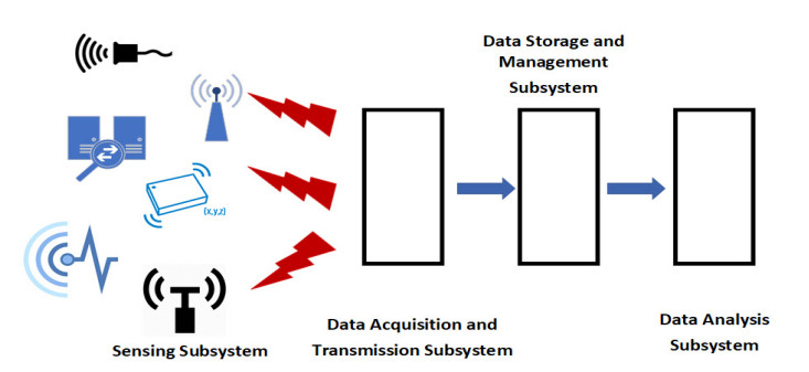
The anti-seismic support and hanger are firmly connected to the building structure and are anti-seismic support equipment with seismic force as the main load. Real-time and accurate acquisition of the service status of the seismic support and hanger to check and judge whether the seismic support and hanger are in a normal working state is of great significance for practical engineering applications. In this paper, based on distributed sensor technology, a set of intelligent monitoring systems for seismic support and hanger of buildings is established. The sensing equipment installed on the seismic support and hanger senses the signal, and then the data collection, storage and processing are used to accurately judge the seismic support and hanger. Service performance status. To effectively fuse multi-source data in distributed sensor environment, an improved method based on wavelet and neural network data fusion is proposed. Compared with the existing methods, the experimental results show that the proposed method has good robustness. Besides, it has better performance in building seismic multi-source monitoring data fusion and is less affected by the data overlap ratio.
Citation: Pingping Chen, Mingyang Qi, Long Chen. Distributed sensors and neural network driven building earthquake resistance mechanism[J]. AIMS Geosciences, 2022, 8(4): 718-730. doi: 10.3934/geosci.2022040
The anti-seismic support and hanger are firmly connected to the building structure and are anti-seismic support equipment with seismic force as the main load. Real-time and accurate acquisition of the service status of the seismic support and hanger to check and judge whether the seismic support and hanger are in a normal working state is of great significance for practical engineering applications. In this paper, based on distributed sensor technology, a set of intelligent monitoring systems for seismic support and hanger of buildings is established. The sensing equipment installed on the seismic support and hanger senses the signal, and then the data collection, storage and processing are used to accurately judge the seismic support and hanger. Service performance status. To effectively fuse multi-source data in distributed sensor environment, an improved method based on wavelet and neural network data fusion is proposed. Compared with the existing methods, the experimental results show that the proposed method has good robustness. Besides, it has better performance in building seismic multi-source monitoring data fusion and is less affected by the data overlap ratio.

| [1] |
Sbarufatti C, Manes A, Giglio M (2014) Application of sensor technologies for local and distributed structural health monitoring. Struct Control Health Monit 21: 1057–1083. https://doi.org/10.1002/stc.1632 doi: 10.1002/stc.1632

|
| [2] |
Ye XW, Su YH, Han JP (2014) Structural health monitoring of civil infrastructure using optical fiber sensing technology: A comprehensive review. Sci World J 2014: 652329. https://doi.org/10.1155/2014/652329 doi: 10.1155/2014/652329
|
| [3] | Goodwin ER (2005) Experimental evaluation of the seismic performance of hospital piping subassemblies. University of Nevada, Reno. |
| [4] |
Zaghi AE, Maragakis EM, Itani A, et al. (2012) Experimental and analytical studies of hospital piping assemblies subjected to seismic loading. Earthquake Spectra 28: 367–384. https://doi.org/10.1193/1.3672911 doi: 10.1193/1.3672911
|
| [5] |
Hoehler MS, Panagiotou M, Restrepo JI, et al. (2009) Performance of suspended pipes and their anchorages during shake table testing of a seven-story building. Earthquake Spectra 25: 71–91. https://doi.org/10.1193/1.3046286 doi: 10.1193/1.3046286
|
| [6] |
Tian Y, Filiatrault A, Mosqueda G (2015) Seismic response of pressurized fire sprinkler piping systems Ⅰ: experimental study. J Earthquake Eng 19: 649–673. https://doi.org/10.1080/13632469.2014.994147 doi: 10.1080/13632469.2014.994147
|
| [7] |
Banerjee TP, Das S (2012) Multi-sensor data fusion using support vector machine for motor fault detection. Inf Sci 217: 96–107. https://doi.org/10.1016/j.ins.2012.06.016 doi: 10.1016/j.ins.2012.06.016
|
| [8] |
Lv Z, Song H (2021) Trust mechanism of feedback trust weight in multimedia network. ACM Trans Multimedia Comput Commun Appl (TOMM) 17: 1–26. https://doi.org/10.1145/3391296 doi: 10.1145/3391296
|
| [9] |
Anees J, Zhang HC, Baig S, et al. (2020) Hesitant fuzzy entropy-based opportunistic clustering and data fusion algorithm for heterogeneous wireless sensor networks. Sensors 20: 913. https://doi.org/10.3390/s20030913 doi: 10.3390/s20030913
|
| [10] | Yang M (2015) Constructing energy efficient data aggregation trees based on information entropy in wireless sensor networks. In 2015 IEEE Advanced Information Technology, Electronic and Automation Control Conference (IAEAC), IEEE, 2015: 527–531. https://doi.org/10.1109/IAEAC.2015.7428609 |
| [11] | Liu CY, Yin XB, Zhang B (2015) Analysis and prediction of landslide deformations based on data fusion technology of Kalman-filter. Chin J Geol Hazard Control 26: 30–35. |
| [12] | Samadzadegan F, Abdi G (2012) Autonomous navigation of Unmanned Aerial Vehicles based on multi-sensor data fusion. In 20th Iranian Conference on Electrical Engineering (ICEE2012), IEEE, 868–873. https://doi.org/10.1109/IranianCEE.2012.6292475 |
| [13] |
Liu F, Liu Y, Sun X, et al. (2021) A new multi-sensor hierarchical data fusion algorithm based on unscented Kalman filter for the attitude observation of the wave glider. Appl Ocean Res 109: 102562. https://doi.org/10.1016/j.apor.2021.102562 doi: 10.1016/j.apor.2021.102562
|
| [14] |
He J, Yang S, Papatheou E, et al. (2019) Investigation of a multi-sensor data fusion technique for the fault diagnosis of gearboxes. Proc Inst Mech Eng Part C J Mech Eng Sci 233: 4764–4775. https://doi.org/10.1177/0954406219834048 doi: 10.1177/0954406219834048
|
| [15] | Chou PH, Hsu YL, Lee WL, et al. (2017) Development of a smart home system based on multi-sensor data fusion technology. In 2017 international conference on applied system innovation (ICASI), IEEE, 690–693. https://doi.org/10.1109/ICASI.2017.7988519 |
| [16] | Medjahed H, Istrate D, Boudy J, et al. (2011) A pervasive multi-sensor data fusion for smart home healthcare monitoring. In 2011 IEEE international conference on fuzzy systems (FUZZ-IEEE 2011), IEEE, 1466–1473. https://doi.org/10.1109/FUZZY.2011.6007636 |
| [17] |
Huang M, Liu Z, Tao Y (2020) Mechanical fault diagnosis and prediction in IoT based on multi-source sensing data fusion. Simul Modell Pract Theory 102: 101981. https://doi.org/10.1016/j.simpat.2019.101981 doi: 10.1016/j.simpat.2019.101981
|
| [18] |
Rawat S, Rawat S (2016) Multi-sensor data fusion by a hybrid methodology–A comparative study. Comput Ind 75: 27–34. https://doi.org/10.1016/j.compind.2015.10.012 doi: 10.1016/j.compind.2015.10.012
|
| [19] |
Al-Sharman MK, Emran BJ, Jaradat MA, et al. (2018) Precision landing using an adaptive fuzzy multi-sensor data fusion architecture. Appl Soft Comput 69: 149–164. https://doi.org/10.1016/j.asoc.2018.04.025 doi: 10.1016/j.asoc.2018.04.025
|
| [20] |
Xiao F (2019) Multi-sensor data fusion based on the belief divergence measure of evidences and the belief entropy. Inf Fusion 46: 23–32. https://doi.org/10.1016/j.inffus.2018.04.003 doi: 10.1016/j.inffus.2018.04.003
|
| [21] |
Majumder S, Pratihar DK (2018) Multi-sensors data fusion through fuzzy clustering and predictive tools. Expert Syst Appl 107: 165–172. https://doi.org/10.1016/j.eswa.2018.04.026 doi: 10.1016/j.eswa.2018.04.026
|
| [22] |
Kumar P, Gauba H, Roy PP, et al. (2017) Coupled HMM-based multi-sensor data fusion for sign language recognition. Pattern Recognit Lett 86: 1–8. https://doi.org/10.1016/j.patrec.2016.12.004 doi: 10.1016/j.patrec.2016.12.004
|
| [23] |
Li G, Yi W, Li S, et al. (2019) Asynchronous multi-rate multi-sensor fusion based on random finite set. Signal Process 160: 113–126. https://doi.org/10.1016/j.sigpro.2019.01.028 doi: 10.1016/j.sigpro.2019.01.028
|
| [24] | Stengel D (2009) System identification for 4 types of structures in Istanbul by frequency domain decomposition and Stochastic subspace identification methods. Diplo-‐ma Thesis, University of Karlsruhe, Karlsruhe, Germany. |
| [25] |
Lu JY, Lin H, Ye D, et al. (2016) A new wavelet threshold function and denoising application. Math Probl Eng 2016: 3195492. https://doi.org/10.1155/2016/3195492 doi: 10.1155/2016/3195492
|
| [26] | Jin W, Li ZJ, Wei LS, et al. (2000) The improvements of BP neural network learning algorithm. In WCC 2000-ICSP 2000. 2000 5th international conference on signal processing proceedings. 16th world computer congress 2000, IEEE, 3: 1647–1649. https://doi.org/10.1109/ICOSP.2000.893417 |


Figures(3) / Tables(2)

Pingping Chen, Mingyang Qi, Long Chen. Distributed sensors and neural network driven building earthquake resistance mechanism[J]. AIMS Geosciences, 2022, 8(4): 718-730. doi: 10.3934/geosci.2022040


 DownLoad: