Resnet-1DCNN-REA bearing fault diagnosis method based on multi-source and multi-modal information fusion

Xu Chen; Wenbing Chang; Yongxiang Li; Zhao He; Xiang Ma; Shenghan Zhou; Xu Chen; Wenbing Chang; Yongxiang Li; Zhao He; Xiang Ma; Shenghan Zhou

doi:10.3934/era.2024292

Electronic Research Archive

2024, Volume 32, Issue 11: 6276-6300. doi: 10.3934/era.2024292

Previous Article Next Article

Research article Special Issues

Resnet-1DCNN-REA bearing fault diagnosis method based on multi-source and multi-modal information fusion

1.
School of Economics and Management, Beihang University, Beijing 100191, China
2.
School of Reliability and Systems Engineering, Beihang University, Beijing 100191, China
3.
Aerospace Information Research Institute, Chinese Academy of Sciences, Beijing 100094, China
† These three authors contributed equally to this work.

Received: 09 July 2024 Revised: 26 October 2024 Accepted: 12 November 2024 Published: 20 November 2024

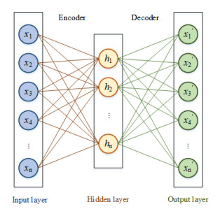
In order to address the issue of multi-information fusion, this paper proposed a method for bearing fault diagnosis based on multisource and multimodal information fusion. Existing bearing fault diagnosis methods mainly rely on single sensor information. Nevertheless, mechanical faults in bearings are intricate and subject to countless excitation disturbances, which poses a great challenge for accurate identification if only relying on feature extraction from single sensor input. In this paper, a multisource information fusion model based on auto-encoder was first established to achieve the fusion of multi-sensor signals. Based on the fused signals, multimodal feature extraction was realized by integrating image features and time-frequency statistical information. The one-dimensional vibration signals were converted into two-dimensional time-frequency images by continuous wavelet transform (CWT), and then they were fed into the Resnet network for fault diagnosis. At the same time, the time-frequency statistical features of the fused 1D signal were extracted from the integrated perspective of time and frequency domains and inputted into the improved 1D convolutional neural network model based on the residual block and attention mechanism (1DCNN-REA) model to realize fault diagnosis. Finally, the tree-structured parzen estimator (TPE) algorithm was utilized to realize the integration of two models in order to improve the diagnostic effect of a single model and obtain the final bearing fault diagnosis results. The proposed model was validated using real experimental data, and the results of the comparison and ablation experiments showed that compared with other models, the proposed model can precisely diagnosis the fault type with an accuracy rate of 98.93%.
- fault diagnosis,
- CNN,
- residual block,
- Resnet,
- bearing fault,
- attention mechanism
Citation: Xu Chen, Wenbing Chang, Yongxiang Li, Zhao He, Xiang Ma, Shenghan Zhou. Resnet-1DCNN-REA bearing fault diagnosis method based on multi-source and multi-modal information fusion[J]. Electronic Research Archive, 2024, 32(11): 6276-6300. doi: 10.3934/era.2024292

Related Papers:

Abstract

In order to address the issue of multi-information fusion, this paper proposed a method for bearing fault diagnosis based on multisource and multimodal information fusion. Existing bearing fault diagnosis methods mainly rely on single sensor information. Nevertheless, mechanical faults in bearings are intricate and subject to countless excitation disturbances, which poses a great challenge for accurate identification if only relying on feature extraction from single sensor input. In this paper, a multisource information fusion model based on auto-encoder was first established to achieve the fusion of multi-sensor signals. Based on the fused signals, multimodal feature extraction was realized by integrating image features and time-frequency statistical information. The one-dimensional vibration signals were converted into two-dimensional time-frequency images by continuous wavelet transform (CWT), and then they were fed into the Resnet network for fault diagnosis. At the same time, the time-frequency statistical features of the fused 1D signal were extracted from the integrated perspective of time and frequency domains and inputted into the improved 1D convolutional neural network model based on the residual block and attention mechanism (1DCNN-REA) model to realize fault diagnosis. Finally, the tree-structured parzen estimator (TPE) algorithm was utilized to realize the integration of two models in order to improve the diagnostic effect of a single model and obtain the final bearing fault diagnosis results. The proposed model was validated using real experimental data, and the results of the comparison and ablation experiments showed that compared with other models, the proposed model can precisely diagnosis the fault type with an accuracy rate of 98.93%.

References

[1]	G. Yu, A concentrated time-frequency analysis tool for bearing fault diagnosis, IEEE Trans. Instrum. Meas., 69 (2020), 371–381. https://doi.org/10.1109/TIM.2019.2901514 doi: 10.1109/TIM.2019.2901514
[2]	Q. Ni, J. C. Ji, K. Feng, B. Halkon, A fault information-guided variational mode decomposition (FIVMD) method for rolling element bearings diagnosis, Mech. Syst. Signal Process., 164 (2022), 108216. https://doi.org/10.1016/j.ymssp.2021.108216 doi: 10.1016/j.ymssp.2021.108216
[3]	L. P. Ji, C. Q. Fu, W. Q. Sun, Soft fault diagnosis of analog circuits based on a resnet with circuit spectrum map, IEEE Trans. Circuits Syst. I Regul. Pap., 68 (2021), 2841–2849. https://doi.org/10.1109/TCSI.2021.3076282 doi: 10.1109/TCSI.2021.3076282
[4]	L. Wen, X. Y. Li, L. Gao, A transfer convolutional neural network for fault diagnosis based on ResNet-50, Neural Comput. Appl., 32 (2020), 6111–6124. https://doi.org/10.1007/s00521-019-04097-w doi: 10.1007/s00521-019-04097-w
[5]	Y. Xu, K. Feng, X. Yan, R. Yan, Q. Ni, B. Sun, et al., CFCNN: A novel convolutional fusion framework for collaborative fault identification of rotating machinery, Inf. Fusion, 95 (2023), 1–16. https://doi.org/10.1016/j.inffus.2023.02.012 doi: 10.1016/j.inffus.2023.02.012
[6]	W. Fu, X. Jiang, B. Li, C. Tan, B. Chen, X. Chen, Rolling bearing fault diagnosis based on 2D time-frequency images and data augmentation technique, Meas. Sci. Technol., 34 (2023). https://doi.org/10.1088/1361-6501/acabdb doi: 10.1088/1361-6501/acabdb
[7]	L. Yuan, D. Lian, X. Kang, Y. Chen, K. Zhai, Rolling bearing fault diagnosis based on convolutional neural network and support vector machine, IEEE Access, 8 (2020), 137395–137406. https://doi.org/10.1109/ACCESS.2020.3012053 doi: 10.1109/ACCESS.2020.3012053
[8]	S. Shao, R. Yan, Y. Lu, P. Wang, R. X. Gao, DCNN-based multi-signal induction motor fault diagnosis, IEEE Trans. Instrum. Meas., 69 (2020), 2658–2669. https://doi.org/10.1109/TIM.2019.2925247 doi: 10.1109/TIM.2019.2925247
[9]	H. Wu, Y. Yang, S. Deng, Q. Wang, H. Song, GADF-VGG16 based fault diagnosis method for HVDC transmission lines, PLoS One, 17 (2022). https://doi.org/10.1371/journal.pone.0274613 doi: 10.1371/journal.pone.0274613
[10]	H. Liang, J. Cao, X. Zhao, Average descent rate singular value decomposition and two-dimensional residual neural network for fault diagnosis of rotating machinery, IEEE Trans. Instrum. Meas., 71 (2022), 1–16. https://doi.org/10.1109/TIM.2022.3170973 doi: 10.1109/TIM.2022.3170973
[11]	J. Zheng, J. Wang, J. Ding, C. Yi, H. Wang, Diagnosis and classification of gear composite faults based on S-transform and improved 2D convolutional neural network, Int. J. Dyn. Control, 12 (2024), 1659–1670. https://doi.org/10.1007/s40435-023-01324-0 doi: 10.1007/s40435-023-01324-0
[12]	Y. Zhang, Z. Cheng, Z. Wu, E. Dong, R. Zhao, G. Lian, Research on electronic circuit fault diagnosis method based on SWT and DCNN-ELM, IEEE Access, 11 (2023), 71301–71313. https://doi.org/10.1109/ACCESS.2023.3292247 doi: 10.1109/ACCESS.2023.3292247
[13]	P. Hu, C. Zhao, J. Huang, T. Song, Intelligent and small samples gear fault detection based on wavelet analysis and improved CNN, Processes, 11 (2023), 2969. https://doi.org/10.3390/pr11102969 doi: 10.3390/pr11102969
[14]	J. Zhao, S. Yang, Q. Li, Y. Liu, X. Gu, W. Liu, A new bearing fault diagnosis method based on signal-to-image mapping and convolutional neural network, Measurement, 176 (2021). https://doi.org/10.1016/j.measurement.2021.109088 doi: 10.1016/j.measurement.2021.109088
[15]	A. Choudhary, R. K. Mishra, S. Fatima, B. K. Panigrahi, Multi-input CNN based vibro-acoustic fusion for accurate fault diagnosis of induction motor, Eng. Appl. Artif. Intell., 120 (2023), 105872. https://doi.org/10.1016/j.engappai.2023.105872 doi: 10.1016/j.engappai.2023.105872
[16]	Z. Hu, Y. Wang, M. Ge, J. Liu, Data-driven fault diagnosis method based on compressed sensing and improved multiscale network, IEEE Trans. Ind. Electron., 67 (2020), 3216–3225. https://doi.org/10.1109/TIE.2019.2912763 doi: 10.1109/TIE.2019.2912763
[17]	D. Ruan, J. Wang, J. Yan, C. Gühmann, CNN parameter design based on fault signal analysis and its application in bearing fault diagnosis, Adv. Eng. Inf., 55 (2023), 101877. https://doi.org/10.1016/j.aei.2023.101877 doi: 10.1016/j.aei.2023.101877
[18]	J. Xiong, M. Liu, C. Li, J. Cen, Q. Zhang, Q. Liu, A bearing fault diagnosis method based on improved mutual dimensionless and deep learning, IEEE Sens. J., 23 (2023), 18338–18348. https://doi.org/10.1109/JSEN.2023.3264870 doi: 10.1109/JSEN.2023.3264870
[19]	J. Zhang, Y. Sun, L. Guo, H. Gao, X. Hong, H. Song, A new bearing fault diagnosis method based on modified convolutional neural networks, Chin. J. Aeronaut., 33 (2020), 439–447. https://doi.org/10.1016/j.cja.2019.07.011 doi: 10.1016/j.cja.2019.07.011
[20]	Y. H. Zhang, T. T. Zhou, X. F. Huang, L. C. Cao, Q. Zhou, Fault diagnosis of rotating machinery based on recurrent neural networks, Measurement, 171 (2021), 108774. https://doi.org/10.1016/j.measurement.2020.108774 doi: 10.1016/j.measurement.2020.108774
[21]	D. Ruan, F. Zhang, C. Gühmann, Exploration and effect analysis of improvement in convolution neural network for bearing fault diagnosis, in Proceedings of the 2021 IEEE International Conference on Prognostics and Health Management (ICPHM), 2021. https://doi.org/10.1109/ICPHM51084.2021.9486665
[22]	L. X. Yang, Z. J. Zhang, A conditional convolutional autoencoder-based method for monitoring wind turbine blade breakages, IEEE Trans. Ind. Inf., 17 (2021), 6390–6398. https://doi.org/10.1109/TII.2020.3011441 doi: 10.1109/TII.2020.3011441
[23]	H. T. Wang, X. W. Liu, L. Y. Ma, Y. Zhang, Anomaly detection for hydropower turbine unit based on variational modal decomposition and deep autoencoder, Energy Rep., 7 (2021), 938–946. https://doi.org/10.1016/j.egyr.2021.09.179 doi: 10.1016/j.egyr.2021.09.179
[24]	H. Y. Zhong, Y. Lv, R. Yuan, D. Yang, Bearing fault diagnosis using transfer learning and self-attention ensemble lightweight convolutional neural network, Neurocomputing, 501 (2022), 765–777. https://doi.org/10.1016/j.neucom.2022.06.066 doi: 10.1016/j.neucom.2022.06.066
[25]	Y. W. Cheng, M. X. Lin, J. Wu, H. P. Zhu, X. Y. Shao, Intelligent fault diagnosis of rotating machinery based on continuous wavelet transform-local binary convolutional neural network, Knowledge-Based Syst., 216 (2021), 106796. https://doi.org/10.1016/j.knosys.2021.106796 doi: 10.1016/j.knosys.2021.106796
[26]	Y. Xu, Z. X. Li, S. Q. Wang, W. H. Li, T. Sarkodie-Gyan, S. Z. Feng, A hybrid deep-learning model for fault diagnosis of rolling bearings, Measurement, 169 (2021), 108502. https://doi.org/10.1016/j.measurement.2020.108502 doi: 10.1016/j.measurement.2020.108502
[27]	L. Han, C. C. Yu, K. T. Xiao, X. Zhao, A new method of mixed gas identification based on a convolutional neural network for time series classification, Sensors, 19 (2019), 1960. https://doi.org/10.3390/s19091960 doi: 10.3390/s19091960
[28]	Y. He, K. Song, Q. Meng, Y. Yan, An end-to-end steel surface defect detection approach via fusing multiple hierarchical features, IEEE Trans. Instrum. Meas., 69 (2020), 1493–1504. https://doi.org/10.1109/TIM.2019.2915404 doi: 10.1109/TIM.2019.2915404
[29]	M. A. Mohammed, K. H. Abdulkareem, S. A. Mostafa, M. K. A. Ghani, M. S. Maashi, B. Garcia-Zapirain, et al., Voice pathology detection and classification using convolutional neural network model, Appl. Sci.-Basel, 10 (2020), 3723. https://doi.org/10.3390/app10113723 doi: 10.3390/app10113723
[30]	Y. Bai, S. Liu, Y. He, L. Cheng, F. Liu, X. Geng, Identification of MOSFET working state based on the stress wave and deep learning, IEEE Trans. Instrum. Meas., 71 (2022), 1–9. https://doi.org/10.1109/TIM.2022.3165276 doi: 10.1109/TIM.2022.3165276
[31]	S. Z. Huang, J. Tang, J. Y. Dai, Y. Y. Wang, Signal status recognition based on 1DCNN and its feature extraction mechanism analysis, Sensors, 19 (2019), 2018. https://doi.org/10.3390/s19092018 doi: 10.3390/s19092018
[32]	M. W. Newcomer, R. J. Hunt, NWTOPT-A hyperparameter optimization approach for selection of environmental model solver settings, Environ. Modell. Software, 147 (2022), 105250. https://doi.org/10.1016/j.envsoft.2021.105250 doi: 10.1016/j.envsoft.2021.105250
[33]	W. Wei, X. Zhao, Bi-TLLDA and CSSVM based fault diagnosis of vehicle on-board equipment for high speed railway, Meas. Sci. Technol., 32 (2021). https://doi.org/10.1088/1361-6501/abe667 doi: 10.1088/1361-6501/abe667

Reader Comments

Your name:*

Email:*
© 2024 the Author(s), licensee AIMS Press. This is an open access article distributed under the terms of the Creative Commons Attribution License (http://creativecommons.org/licenses/by/4.0)