Faster free pseudoinverse greedy block Kaczmarz method for image recovery

Wenya Shi; Xinpeng Yan; Zhan Huan; Wenya Shi; Xinpeng Yan; Zhan Huan

doi:10.3934/era.2024178

Electronic Research Archive

2024, Volume 32, Issue 6: 3973-3988. doi: 10.3934/era.2024178

Previous Article Next Article

Research article Special Issues

Faster free pseudoinverse greedy block Kaczmarz method for image recovery

Aliyun Big Data College, Changzhou University, Changzhou 213159, China

Received: 09 April 2024 Revised: 22 May 2024 Accepted: 31 May 2024 Published: 17 June 2024

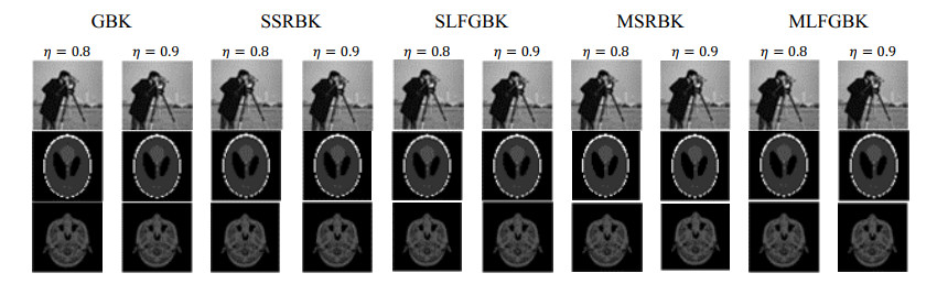
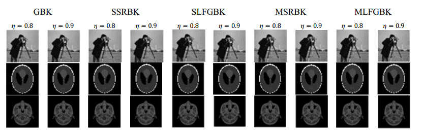
The greedy block Kaczmarz (GBK) method has been successfully applied in areas such as data mining, image reconstruction, and large-scale image restoration. However, the computation of pseudo-inverses in each iterative step of the GBK method not only complicates the computation and slows down the convergence rate, but it is also ill-suited for distributed implementation. The leverage score sampling free pseudo-inverse GBK algorithm proposed in this paper demonstrated significant potential in the field of image reconstruction. By ingeniously transforming the problem framework, the algorithm not only enhanced the efficiency of processing systems of linear equations with multiple solution vectors but also optimized specifically for applications in image reconstruction. A methodology that combined theoretical and experimental approaches has validated the robustness and practicality of the algorithm, providing valuable insights for technical advancements in related disciplines.
- leverage score sampling,
- greedy block Kaczmarz method,
- free pseudo-inverse,
- multiple righthand sides,
- image recovery
Citation: Wenya Shi, Xinpeng Yan, Zhan Huan. Faster free pseudoinverse greedy block Kaczmarz method for image recovery[J]. Electronic Research Archive, 2024, 32(6): 3973-3988. doi: 10.3934/era.2024178

Related Papers:

Abstract

The greedy block Kaczmarz (GBK) method has been successfully applied in areas such as data mining, image reconstruction, and large-scale image restoration. However, the computation of pseudo-inverses in each iterative step of the GBK method not only complicates the computation and slows down the convergence rate, but it is also ill-suited for distributed implementation. The leverage score sampling free pseudo-inverse GBK algorithm proposed in this paper demonstrated significant potential in the field of image reconstruction. By ingeniously transforming the problem framework, the algorithm not only enhanced the efficiency of processing systems of linear equations with multiple solution vectors but also optimized specifically for applications in image reconstruction. A methodology that combined theoretical and experimental approaches has validated the robustness and practicality of the algorithm, providing valuable insights for technical advancements in related disciplines.

References

[1]	A. C. Kak, M. Slaney, Principles of computerized tomographic imaging, Society for Industrial and Applied Mathematics, New York, 2001.
[2]	J. A. Fessler, B. P. Sutton, Nonuniform fast Fourier transforms using min-max interpolation, IEEE T. Signal Proces., 51 (2003), 560–574. https://doi.org/10.1109/TSP.2002.807005 doi: 10.1109/TSP.2002.807005
[3]	S. F. Gull, G. J. Daniell, Image reconstruction from incomplete and noisy data, Nature, 272 (1978), 686–690. https://doi.org/10.1038/272686a0 doi: 10.1038/272686a0
[4]	X. L. Zhao, T. Z. Huang, X. M. Gu, L. J. Deng, Vector extrapolation based Landweber method for discrete ill-posed problems, Math. Probl. Eng., 2017 (2017), 1375716. https://doi.org/10.1155/2017/1375716 doi: 10.1155/2017/1375716
[5]	S. C. Park, M. K. Park, M. G. Kang, Super-resolution image reconstruction: a technical overview, IEEE Signal Proc. Mag., 20 (2003), 21–36. https://doi.org/10.1109/MSP.2003.120320 doi: 10.1109/MSP.2003.120320
[6]	F. Natterer, F. Wübbeling, Mathematical methods in image reconstruction, Society for Industrial and Applied Mathematics, New York, 2001.
[7]	G. L. Zeng, Image reconstruction—a tutorial, Comput. Med. Imag. Grap., 25 (2001), 97–103. https://doi.org/10.1016/S0895-6111(00)00059-8 doi: 10.1016/S0895-6111(00)00059-8
[8]	J. I. Goldstein, D. E. Newbury, J. R. Michael, N. W. M. Ritchie, J. H. J. Scott, D. C. Joy, X-Rays, in Scanning Electron Microscopy and X-Ray Microanalysis, Springer, (2018), 39–63. https://doi.org/10.1007/978-1-4939-6676-9_4
[9]	P. Toft, The Radon Transform-Theory and Implementation, Ph.D thesis, Technical University of Denmark in Copenhagen, 1996.
[10]	A. Rahman, System of linear equations in Computed Tomography (CT), Bachelor's thesis, Brac University in Dacca, 2018.
[11]	G. T. Herman, Fundamentals of Computerized Tomography: Image Reconstruction from Projections, Springer Science & Business Media, Berlin, 2009.
[12]	Y. Censor, G. T. Herman, M. Jiang, A note on the behavior of the randomized Kaczmarz algorithm of Strohmer and Vershynin, J. Fourier Anal. Appl., 15 (2009), 431–436. https://doi.org/10.1007/s00041-009-9077-x doi: 10.1007/s00041-009-9077-x
[13]	O. Axelsson, Iterative Solution Methods, Cambridge University Press, Cambridge, 1996.
[14]	I. Gohberg, I. A. Fel_dman, Convolution Equations and Projection Methods for Their Solution, American Mathematical Soc., Providence, 2005.
[15]	Z. Z. Bai, C. H. Jin, Column-decomposed relaxation methods for the overdetermined systems of linear equations, Int. J. Appl. Mat. Com.-Pol., 13 (2003), 71–82.
[16]	S. Kaczmarz, Angenäherte auflösung von systemen linearer glei-chungen, Bull. Int. Acad. Pol. Sci. Lett. Class. Sci. Math. Nat., (1937), 355–357.
[17]	M. Brooks, A Survey of Algebraic Algorithms in Computerized Tomography, Master's Thesis, University of Ontario Institute of Technology in Oshawa, 2010.
[18]	Y. Censor, Parallel application of block-iterative methods in medical imaging and radiation therapy, Math. Program., 42 (1988), 307–325. https://doi.org/10.1007/BF01589408 doi: 10.1007/BF01589408
[19]	C. Byrne, A unified treatment of some iterative algorithms in signal processing and image reconstruction, Inverse Probl., 20 (20031), 103. https://doi.org/10.1088/0266-5611/20/1/006 doi: 10.1088/0266-5611/20/1/006
[20]	D. A. Lorenz, S. Wenger, F. Schöpfer, M. Magnor, A sparse Kaczmarz solver and a linearized Bregman method for online compressed sensing, in 2014 IEEE International Conference on Image Processing (ICIP), (2014), 1347–1351. https://doi.org/10.1109/ICIP.2014.7025269
[21]	J. D. Moorman, T. K. Tu, D. Molitor, D. Needell, Randomized Kaczmarz with averaging, BIT Numer. Math., 61 (2021), 337–359. https://doi.org/10.1007/s10543-020-00824-1 doi: 10.1007/s10543-020-00824-1
[22]	T. Strohmer, R. Vershynin, A randomized Kaczmarz algorithm with exponential convergence, J. Fourier Anal. Appl., 15 (2009), 262–278. https://doi.org/10.1007/s00041-008-9030-4 doi: 10.1007/s00041-008-9030-4
[23]	A. Zouzias, N. M. Freris, Randomized extended Kaczmarz for solving least squares, SIAM J. Matrix Anal. A., 34 (2013), 773–793.
[24]	K. Du, X. H. Sun, Pseudoinverse-free randomized block iterative algorithms for consistent and inconsistent linear systems, preprint, arXiv: 2011.10353.
[25]	D. Needell, J. A. Tropp, Paved with good intentions: analysis of a randomized block Kaczmarz method, Linear Algebra Appl., 441 (2014), 199–221. https://doi.org/10.1016/j.laa.2012.12.022 doi: 10.1016/j.laa.2012.12.022
[26]	Z Z. Bai, W. T. Wu, On relaxed greedy randomized Kaczmarz methods for solving large sparse linear systems, Appl. Math. Lett., 83 (2018), 21–26. https://doi.org/10.1016/j.aml.2018.03.008 doi: 10.1016/j.aml.2018.03.008
[27]	Z Z. Bai, W. T. Wu, On greedy randomized Kaczmarz method for solving large sparse linear systems, SIAM J. Sci. Comput., 40 (2018), A592–A606. https://doi.org/10.1137/17M1137747 doi: 10.1137/17M1137747
[28]	E. Rebrova, D. Needell, On block Gaussian sketching for the Kaczmarz method, Numer. Algor., 86 (2021), 443–473. https://doi.org/10.1007/s11075-020-00895-9 doi: 10.1007/s11075-020-00895-9
[29]	Y. Q. Niu, B. Zheng, A greedy block Kaczmarz algorithm for solving large-scale linear systems, Appl. Math. Lett., 104 (2020), 106294. https://doi.org/10.1016/j.aml.2020.106294 doi: 10.1016/j.aml.2020.106294
[30]	I. Necoara, Faster randomized block Kaczmarz algorithms, SIAM J. Matrix Anal. A., 40 (2019), 1425–1452. https://doi.org/10.1137/19M1251643 doi: 10.1137/19M1251643
[31]	T. Elfving, Block-iterative methods for consistent and inconsistent linear equations, Numer. Math., 35 (1980), 1–12. https://doi.org/10.1007/BF01396365 doi: 10.1007/BF01396365
[32]	D. P. Woodruff, Sketching as a tool for numerical linear algebra, Found. Trends Theor. Comput. Sci., 10 (2014), 1–157. http://doi.org/10.1561/0400000060 doi: 10.1561/0400000060
[33]	Y. Zhang, H. Li, L. Tang, Greedy randomized sampling nonlinear Kaczmarz methods, Calcolo, 61 (2024). https://doi.org/10.1007/s10092-024-00577-1 doi: 10.1007/s10092-024-00577-1
[34]	J. Zhang, Y. Wang, J. Zhao, On maximum residual nonlinear Kaczmarz-type algorithms for large nonlinear systems of equations, J. Comput. Appl. Math., 425 (2023), 115065. https://doi.org/10.1016/j.cam.2023.115065 doi: 10.1016/j.cam.2023.115065
[35]	T. Li, T. J. Kao, D. Isaacson, J. C. Newell, G. J. Saulnier, Adaptive Kaczmarz method for image reconstruction in electrical impedance tomography, Physiol. Meas., 34 (2013), 595. https://doi.org/10.1088/0967-3334/34/6/595 doi: 10.1088/0967-3334/34/6/595
[36]	M. B. Cohen, C. Musco, C. Musco, Input sparsity time low-rank approximation via ridge leverage score sampling, in Proceedings of the Twenty-Eighth Annual ACM-SIAM Symposium on Discrete Algorithms, (2017), 1758–1777. https://doi.org/10.1137/1.9781611974782.115
[37]	A. Rudi, D. Calandriello, L. Carratino, L. Rosasco, On fast leverage score sampling and optimal learning, Adv. Neural Inform. Process. Syst., 31 (2018).
[38]	Y. Zhang, H. Li, A count sketch maximal weighted residual Kaczmarz method for solving highly overdetermined linear systems, Appl. Math. Comput., 410 (2021), 126486. https://doi.org/10.1016/j.amc.2021.126486 doi: 10.1016/j.amc.2021.126486
[39]	Y. Jiang, G. Wu, L. Jiang, A semi-randomized Kaczmarz method with simple random sampling for large-scale linear systems, Adv. Comput. Math., 49 (2023). https://doi.org/10.1007/s10444-023-10018-2 doi: 10.1007/s10444-023-10018-2
[40]	G. Wu, Q. Chang, A semi-randomized block Kaczmarz method with simple random sampling for large-scale linear systems with multiple right-hand sides, preprint, arXiv: 2212.08797.

Reader Comments

Your name:*

Email:*
© 2024 the Author(s), licensee AIMS Press. This is an open access article distributed under the terms of the Creative Commons Attribution License (http://creativecommons.org/licenses/by/4.0)