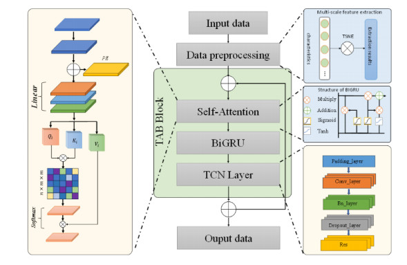
Accurate and effective building energy consumption prediction is an important basis for carrying out energy-saving evaluation and the main basis for building energy-saving optimization design. However, due to the influence of environmental and human factors, energy consumption prediction is often inaccurate. Therefore, this paper presents a building energy consumption prediction model based on an attention mechanism, time convolutional neural (TCN) network fusion, and a bidirectional gated cycle unit (BIGRU). First, t-distributed stochastic neighbor embedding (T-SNE) was used to preprocess the data and extract the key features, and then a BIGRU was employed to acquire past and future data while capturing immediate connections. Then, to catch the long-term dependence, the dataset was partitioned into the TCN network, and the extended sequence was transformed into several short sequences. Consequently, the gradient explosion or vanishing problem is mitigated when the BIGRU handles lengthy sequences while reducing the spatial complexity. Second, the self-attention mechanism was introduced to enhance the model's capability to address data periodicity. The proposed model is superior to the other four models in accuracy, with an mean absolute error of 0.023, an mean-square error of 0.029, and an coefficient of determination of 0.979. Experimental results indicate that T-SNE can significantly improve the model performance, and the accuracy of predictions can be improved by the attention mechanism and the TCN network.
Citation: Yi Deng, Zhanpeng Yue, Ziyi Wu, Yitong Li, Yifei Wang. TCN-Attention-BIGRU: Building energy modelling based on attention mechanisms and temporal convolutional networks[J]. Electronic Research Archive, 2024, 32(3): 2160-2179. doi: 10.3934/era.2024098
Accurate and effective building energy consumption prediction is an important basis for carrying out energy-saving evaluation and the main basis for building energy-saving optimization design. However, due to the influence of environmental and human factors, energy consumption prediction is often inaccurate. Therefore, this paper presents a building energy consumption prediction model based on an attention mechanism, time convolutional neural (TCN) network fusion, and a bidirectional gated cycle unit (BIGRU). First, t-distributed stochastic neighbor embedding (T-SNE) was used to preprocess the data and extract the key features, and then a BIGRU was employed to acquire past and future data while capturing immediate connections. Then, to catch the long-term dependence, the dataset was partitioned into the TCN network, and the extended sequence was transformed into several short sequences. Consequently, the gradient explosion or vanishing problem is mitigated when the BIGRU handles lengthy sequences while reducing the spatial complexity. Second, the self-attention mechanism was introduced to enhance the model's capability to address data periodicity. The proposed model is superior to the other four models in accuracy, with an mean absolute error of 0.023, an mean-square error of 0.029, and an coefficient of determination of 0.979. Experimental results indicate that T-SNE can significantly improve the model performance, and the accuracy of predictions can be improved by the attention mechanism and the TCN network.

| [1] |
D. Li, M. Qiu, J. Jiang, S. Yang, The application of an optimized fractional order accumulated grey model with variable parameters in the total energy consumption of Jiangsu Province and the consumption level of Chinese residents, Electron. Res. Arch., 30 (2022), 798–812. https://doi.org/10.3934/era.2022042 doi: 10.3934/era.2022042

|
| [2] |
M. Aydin, N. I. Mahmudov, H. Aktuğlu, E. Baytunç, M. S. Atamert, On a study of the representation of solutions of a ψ-Caputo fractional differential equations with a single delay, Electron. Res. Arch., 30 (2022), 1016–1034. https://doi.org/10.3934/era.2022053 doi: 10.3934/era.2022053
|
| [3] |
C. Ohajunwa, C. Caiseda, P. Seshaiyer, Computational modeling, analysis and simulation for lockdown dynamics of COVID-19 and domestic violence, Electron. Res. Arch., 30 (2022), 2446–2464. https://doi.org/10.3934/era.2022125 doi: 10.3934/era.2022125
|
| [4] |
J. Zheng, Y. Li, Machine learning model of tax arrears prediction based on knowledge graph, Electron. Res. Arch., 31 (2023), 4057–4076. https://doi.org/10.3934/era.2023206 doi: 10.3934/era.2023206
|
| [5] |
X. Shen, P. Raksincharoensak, Statistical models of near-accident event and pedestrian behavior at non-signalized intersections, J. Appl. Stat., 49 (2022), 4028–4048. https://doi.org/10.1080/02664763.2021.1962263 doi: 10.1080/02664763.2021.1962263
|
| [6] |
Q. Li, D. Huang, S. Pei, J. Qiao, M. Wang, Using physical model experiments for hazards assessment of rainfall-induced debris landslides, J. Earth Sci., 32 (2021), 1113–1128. https://doi.org/10.1007/s12583-020-1398-3 doi: 10.1007/s12583-020-1398-3
|
| [7] |
L. Xu, F. Chen, F. Ding, A. Alsaedi, T. Hayat, Hierarchical recursive signal modeling for multifrequency signals based on discrete measured data, Int. J. Adapt. Control Signal Process., 35 (2021), 676–693. https://doi.org/10.1002/acs.3221 doi: 10.1002/acs.3221
|
| [8] |
D. Alita, A. D. Putra, D. Darwis, Analysis of classic assumption test and multiple linear regression coefficient test for employee structural office recommendation, Indones. J. Comput. Cybern. Syst., 15 (2021), 295–306. https://doi.org/10.22146/ijccs.65586 doi: 10.22146/ijccs.65586
|
| [9] |
M. Hosseinzadeh, A. M. Rahmani, B. Vo, M. Bidaki, M. Masdari, M. Zangakani, Improving security using SVM-based anomaly detection: issues and challenges, Soft Comput., 25 (2021), 3195–3223. https://doi.org/10.1007/s00500-020-05373-x doi: 10.1007/s00500-020-05373-x
|
| [10] |
S. Georganos, T. Grippa, A. N. Gadiaga, C. Linard, M. Lennert, S. Vanhuysse, et al., Geographical random forests: a spatial extension of the random forest algorithm to address spatial heterogeneity in remote sensing and population modelling, Geocarto Int., 36 (2021), 121–136. https://doi.org/10.1080/10106049.2019.1595177 doi: 10.1080/10106049.2019.1595177
|
| [11] |
H. Liu, T. Liu, Y. Chen, Z. Zhang, Y. Li, EHPE: Skeleton cues-based gaussian coordinate encoding for efficient human pose estimation, IEEE Trans. Multimedia, (2022), 1–12. https://doi.org/10.1109/TMM.2022.3197364 doi: 10.1109/TMM.2022.3197364
|
| [12] |
H. Liu, C. Zhang, Y. Deng, T. Liu, Z. Zhang, Y. Li, Orientation cues-aware facial relationship representation for head pose estimation via transformer, IEEE Trans. Image Process., 32 (2023), 6289–6302. https://doi.org/10.1109/TIP.2023.3331309 doi: 10.1109/TIP.2023.3331309
|
| [13] |
H. Liu, C. Zhang, Y. Deng, B. Xie, T. Liu, Z. Zhang, et al., Trans-IFC: Invariant cues aware feature concentration learning for efficient fine-grained bird image classification, IEEE Trans. Multimedia, (2023), 1–14. https://doi.org/10.1109/TMM.2023.3238548 doi: 10.1109/TMM.2023.3238548
|
| [14] |
C. Bentéjac, A. Csörgő, G. Martínez-Muñoz, A comparative analysis of gradient boosting algorithms, Artif. Intell. Rev., 54 (2021), 1937–1967. https://doi.org/10.1007/s10462-020-09896-5 doi: 10.1007/s10462-020-09896-5
|
| [15] |
N. S. Kiruthika, D. G. Thaila, Dynamic light weight recommendation system for social networking analysis using a hybrid LSTM-SVM classifier algorithm, Opt. Mem. Neural Networks, 31 (2022), 59–75. https://doi.org/10.3103/S1060992X2201009X doi: 10.3103/S1060992X2201009X
|
| [16] |
S. Li, Z. Fan, Evaluation of urban green space landscape planning scheme based on PSO-BP neural network model, Alexandria Eng. J., 61 (2022), 7141–7153. https://doi.org/10.1016/j.aej.2021.12.057 doi: 10.1016/j.aej.2021.12.057
|
| [17] |
H. Hewamalage, C. Bergmeir, K. Bandara, Recurrent neural networks for time series forecasting: Current status and future directions, Int. J. Forecast., 37 (2021), 388–427. https://doi.org/10.1016/j.ijforecast.2020.06.008 doi: 10.1016/j.ijforecast.2020.06.008
|
| [18] |
I. Priyadarshini, C. Cotton, A novel LSTM-CNN-grid search-based deep neural network for sentiment analysis, J. Supercomput., 77 (2021), 13911–13932. https://doi.org/10.1007/s11227-021-03838-w doi: 10.1007/s11227-021-03838-w
|
| [19] |
N. Aslam, F. Rustam, E. Lee, P. B. Washington, I. Ashraf, Sentiment analysis and emotion detection on cryptocurrency related tweets using ensemble LSTM-GRU model, IEEE Access, 10 (2022), 39313–39324. https://doi.org/10.1109/ACCESS.2022.3165621 doi: 10.1109/ACCESS.2022.3165621
|
| [20] |
M. Li, D. Xu, J. Geng, W. Hong, A ship motion forecasting approach based on empirical mode decomposition method hybrid deep learning network and quantum butterfly optimization algorithm, Nonlinear Dyn., 107 (2022), 2447–2467. https://doi.org/10.1007/s11071-021-07139-y doi: 10.1007/s11071-021-07139-y
|
| [21] |
Z. Niu, G. Zhong, H. Yu, A review on the attention mechanism of deep learning, Neurocomputing, 452 (2021), 48–62. https://doi.org/10.1016/j.neucom.2021.03.091 doi: 10.1016/j.neucom.2021.03.091
|
| [22] |
V. Bagal, R. Aggarwal, P. K. Vinod, U. D. Priyakumar, MolGPT: Molecular generation using a transformer-decoder model, J. Chem. Inf. Model., 62 (2021), 2064–2076. https://doi.org/10.1021/acs.jcim.1c00600 doi: 10.1021/acs.jcim.1c00600
|
| [23] |
Y. Yuan, Z. Chen, Z. Wang, Y. Sun, Y. Chen, Attention mechanism-based transfer learning model for day-ahead energy demand forecasting of shopping mall buildings, Energy, 270 (2023), 126878. https://doi.org/10.1016/j.energy.2023.126878 doi: 10.1016/j.energy.2023.126878
|
| [24] |
D. Kobak, G. C. Linderman, Initialization is critical for preserving global data structure in both t-SNE and UMAP, Nat. Biotechnol., 39 (2021), 156–157. https://doi.org/10.1038/s41587-020-00809-z doi: 10.1038/s41587-020-00809-z
|
| [25] |
T. Ahmad, H. Chen, Y. Guo, J. Wang, A comprehensive overview on the data driven and large scale based approaches for forecasting of building energy demand: A review, Energy Build., 165 (2018), 301–320. https://doi.org/10.1016/j.enbuild.2018.01.017 doi: 10.1016/j.enbuild.2018.01.017
|
| [26] |
T. Liu, H. Liu, B. Yang, Z. Zhang, Limb direction cues-aware network for flexible human pose estimation in industrial behavioral biometrics systems, IEEE Trans. Ind. Inf., (2023), 1–11. https://doi.org/10.1109/TⅡ.2023.3266366 doi: 10.1109/TⅡ.2023.3266366
|
| [27] |
H. Liu, T. Liu, Z. Zhang, A. K. Sanga, B. Yang, Y. Li, ARHPE: Asymmetric relation-aware representation learning for head pose estimation in industrial human-computer interaction, IEEE Trans. Ind. Inf., 18 (2022), 7107–7117. https://doi.org/10.1109/TⅡ.2022.3143605 doi: 10.1109/TⅡ.2022.3143605
|
| [28] |
H. Liu, S. Fang, Z. Zhang, D. Li, K. Lin, J. Wang, MFDNET: Collaborative poses perception and matrix fisher distribution for head pose estimation, IEEE Trans. Multimedia, 24 (2021), 2449–2460. https://doi.org/10.1109/TMM.2021.3081873 doi: 10.1109/TMM.2021.3081873
|
| [29] |
H. Liu, C. Zheng, D. Li, X. Shen, K. Lin, J. Wang, et al., EDMF: Efficient deep matrix factorization with review feature learning for industrial recommender system, IEEE Trans. Ind. Inf., 18 (2022), 4361–4371. https://doi.org/10.1109/TⅡ.2021.3128240 doi: 10.1109/TⅡ.2021.3128240
|
| [30] |
D. Liu, W. Wang, X. Wang, C. Wang, J. Pei, W. Chen, Posts seismic data denoising based on 3-D convolutional neural network, IEEE Trans. Geosci. Remote Sens., 58 (2020), 1598–1629. https://doi.org/10.1109/TGRS.2019.2947149 doi: 10.1109/TGRS.2019.2947149
|
| [31] |
A. Daffertshofer, C. J. C. Lamoth, O. G. Meijer, P. J. Beek, PCA in studying coordination and variability: a tutorial, Clin. Biomech., 19 (2004): 415–428. https://doi.org/10.1016/j.clinbiomech.2004.01.005 doi: 10.1016/j.clinbiomech.2004.01.005
|
| [32] |
L. Gao, J. Gao, J. Li, A. Plaza, L. Zhuang, X. Sun, et al., Multiple algorithm integration based on ant colony optimization for endmember extraction from hyperspectral imagery, IEEE J. Sel. Top. Appl. Earth Obs. Remote Sens., 8 (2014), 2569–2582. https://doi.org/10.1109/JSTARS.2014.2371615 doi: 10.1109/JSTARS.2014.2371615
|
| [33] |
P. Hewage, A. Behera, M. Trovati, E. Pereira, M. Ghahremani, F. Palmieri, et al., Temporal convolutional neural (TCN) network for an effective weather forecasting using time-series data from the local weather station, Soft Comput., 24 (2020), 16453–16482. https://doi.org/10.1007/s00500-020-04954-0 doi: 10.1007/s00500-020-04954-0
|
| [34] |
Y. Yu, L. You, D. Liu, W. Hollinshead, Y. J. Tang, F. Zhang, Development of Syne sp. PCC 6803 as a phototrophic cell factory, Mar. Drugs, 11 (2013), 2894–2916. https://doi.org/10.3390/md11082894 doi: 10.3390/md11082894
|
| [35] |
A. K. Shahade, K. H. Walse, V. M. Thakare, Deep learning approach-based hybrid fine-tuned Smith algorithm with Adam optimiser for multilingual opinion mining, Int. J. Comput. Appl. Technol., 73 (2023), 50–65. https://doi.org/10.1504/IJCAT.2023.134080 doi: 10.1504/IJCAT.2023.134080
|
| [36] |
H. Liu, C. Zheng, D. Li, Z. Zhang, K. Lin, X. Shen, et al., Multi-perspective social recommendation method with graph representation learning, Neurocomputing, 468 (2022), 469–481. https://doi.org/10.1016/j.neucom.2021.10.050 doi: 10.1016/j.neucom.2021.10.050
|
| [37] |
B. A. Draper, K. Baek, M. S. Bartlett, J. R. Beveridge, Recognizing faces with PCA and ICA, Comput. Vision Image Understanding, 91 (2003), 115–137. https://doi.org/10.1016/S1077-3142(03)00077-8 doi: 10.1016/S1077-3142(03)00077-8
|


Figures(8) / Tables(7)
Yi Deng, Zhanpeng Yue, Ziyi Wu, Yitong Li, Yifei Wang. TCN-Attention-BIGRU: Building energy modelling based on attention mechanisms and temporal convolutional networks[J]. Electronic Research Archive, 2024, 32(3): 2160-2179. doi: 10.3934/era.2024098


 DownLoad: