In the digital era, human-robot interaction is rapidly expanding, emphasizing the need for social robots to fluently understand and communicate in multiple languages. It is not merely about decoding words but about establishing connections and building trust. However, many current social robots are limited to popular languages, serving in fields like language teaching, healthcare and companionship. This review examines the AI-driven language abilities in social robots, providing a detailed overview of their applications and the challenges faced, from nuanced linguistic understanding to data quality and cultural adaptability. Last, we discuss the future of integrating advanced language models in robots to move beyond basic interactions and towards deeper emotional connections. Through this endeavor, we hope to provide a beacon for researchers, steering them towards a path where linguistic adeptness in robots is seamlessly melded with their capacity for genuine emotional engagement.
Citation: Yanling Dong, Xiaolan Zhou. Advancements in AI-driven multilingual comprehension for social robot interactions: An extensive review[J]. Electronic Research Archive, 2023, 31(11): 6600-6633. doi: 10.3934/era.2023334
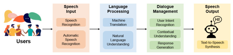
In the digital era, human-robot interaction is rapidly expanding, emphasizing the need for social robots to fluently understand and communicate in multiple languages. It is not merely about decoding words but about establishing connections and building trust. However, many current social robots are limited to popular languages, serving in fields like language teaching, healthcare and companionship. This review examines the AI-driven language abilities in social robots, providing a detailed overview of their applications and the challenges faced, from nuanced linguistic understanding to data quality and cultural adaptability. Last, we discuss the future of integrating advanced language models in robots to move beyond basic interactions and towards deeper emotional connections. Through this endeavor, we hope to provide a beacon for researchers, steering them towards a path where linguistic adeptness in robots is seamlessly melded with their capacity for genuine emotional engagement.

| [1] | O. Mubin, J. Henderson, C. Bartneck, You just do not understand me! Speech recognition in human robot interaction, in The 23rd IEEE International Symposium on Robot and Human Interactive Communication, (2014), 637–642. https://doi.org/10.1109/ROMAN.2014.6926324 |
| [2] |
T. Belpaeme, J. Kennedy, A. Ramachandran, B. Scassellati, F. Tanaka, Social robots for education: a review, Sci. Rob., 3 (2018), eaat5954. https://doi.org/10.1126/scirobotics.aat5954 doi: 10.1126/scirobotics.aat5954

|
| [3] |
Y. Wang, S. Zhong, G. Wang, Preventing online disinformation propagation: cost-effective dynamic budget allocation of refutation, media censorship, and social bot detection, Math. Biosci. Eng., 20 (2023), 13113–13132. https://doi.org/10.3934/mbe.2023584 doi: 10.3934/mbe.2023584
|
| [4] |
C. A. Cifuentes, M. J. Pinto, N. Céspedes, M. Múnera, Social robots in therapy and care, Curr. Rob. Rep., 1 (2020), 59–74. https://doi.org/10.1007/s43154-020-00009-2 doi: 10.1007/s43154-020-00009-2
|
| [5] |
H. Su, W. Qi, J. Chen, D. Zhang, Fuzzy approximation-based task-space control of robot manipulators with remote center of motion constraint, IEEE Trans. Fuzzy Syst., 30 (2022), 1564–1573. https://doi.org/10.1109/TFUZZ.2022.3157075 doi: 10.1109/TFUZZ.2022.3157075
|
| [6] |
J. Hirschberg, C. D. Manning, Advances in natural language processing, Science, 349 (2015), 261–266. https://doi.org/10.1126/science.aaa8685 doi: 10.1126/science.aaa8685
|
| [7] | S. H. Paplu, K. Berns, Towards linguistic and cognitive competence for socially interactive robots, in Robot Intelligence Technology and Applications 6, Springer, (2021), 520–530. https://doi.org/10.1007/978-3-030-97672-9_47 |
| [8] |
E. B. Onyeulo, V. Gandhi, What makes a social robot good at interacting with humans? Information, 11 (2020), 43. https://doi.org/10.3390/info11010043 doi: 10.3390/info11010043
|
| [9] |
C. Ke, V. W. Lou, K. C. Tan, M. Y. Wai, L. L. Chan, Changes in technology acceptance among older people with dementia: the role of social robot engagement, Int. J. Med. Inf., 141 (2020), 104241. https://doi.org/10.1016/j.ijmedinf.2020.104241 doi: 10.1016/j.ijmedinf.2020.104241
|
| [10] | Y. Kim, H. Chen, S. Alghowinem, C. Breazeal, H. W. Park, Joint engagement classification using video augmentation techniques for multi-person human-robot interaction, preprint, arXiv: 2212.14128. |
| [11] |
A. A. Allaban, M. Wang, T. Padır, A systematic review of robotics research in support of in-home care for older adults, Information, 11 (2020), 75. https://doi.org/10.3390/info11020075 doi: 10.3390/info11020075
|
| [12] |
W. Qi, A. Aliverti, A multimodal wearable system for continuous and real-time breathing pattern monitoring during daily activity, IEEE J. Biomed. Health. Inf., 24 (2019), 2199–2207. https://doi.org/10.1109/JBHI.2019.2963048 doi: 10.1109/JBHI.2019.2963048
|
| [13] |
C. Barras, Could speech recognition improve your meetings? New Sci., 205 (2010), 18–19. https://doi.org/10.1016/S0262-4079(10)60347-8 doi: 10.1016/S0262-4079(10)60347-8
|
| [14] | Y. J. Lu, X. Chang, C. Li, W. Zhang, S. Cornell, Z. Ni, et al., Espnet-se++: Speech enhancement for robust speech recognition, translation, and understanding, preprint, arXiv: 2207.09514. |
| [15] |
L. Besacier, E. Barnard, A. Karpov, T. Schultz, Automatic speech recognition for under-resourced languages: a survey, Speech Commun., 56 (2014), 85–100. https://doi.org/10.1016/j.specom.2013.07.008 doi: 10.1016/j.specom.2013.07.008
|
| [16] | G. I. Winata, S. Cahyawijaya, Z. Liu, Z. Lin, A. Madotto, P. Xu, et al., Learning fast adaptation on cross-accented speech recognition, preprint, arXiv: 2003.01901. |
| [17] | S. Kim, B. Raj, I. Lane, Environmental noise embeddings for robust speech recognition, preprint, arXiv: 1601.02553. |
| [18] | A. F. Daniele, M. Bansal, M. R. Walter, Navigational instruction generation as inverse reinforcement learning with neural machine translation, in Proceedings of the 2017 ACM/IEEE International Conference on Human-Robot Interaction, (2017), 109–118. https://doi.org/10.1145/2909824.3020241 |
| [19] |
Z. Liu, D. Yang, Y. Wang, M. Lu, R. Li, Egnn: Graph structure learning based on evolutionary computation helps more in graph neural networks, Appl. Soft Comput., 135 (2023), 110040. https://doi.org/10.1016/j.asoc.2023.110040 doi: 10.1016/j.asoc.2023.110040
|
| [20] |
Y. Wang, Z. Liu, J. Xu, W. Yan, Heterogeneous network representation learning approach for Ethereum identity identification, IEEE Trans. Comput. Social Syst., 10 (2022), 890–899. https://doi.org/10.1109/TCSS.2022.3164719 doi: 10.1109/TCSS.2022.3164719
|
| [21] |
J. Zhao, Y. Lv, Output-feedback robust tracking control of uncertain systems via adaptive learning, Int. J. Control Autom. Syst, 21 (2023), 1108–1118. https://doi.org/10.1007/s12555-021-0882-6 doi: 10.1007/s12555-021-0882-6
|
| [22] |
S. Islam, A. Paul, B. S. Purkayastha, I. Hussain, Construction of English-bodo parallel text corpus for statistical machine translation, Int. J. Nat. Lang. Comput., 7 (2018), 93–103. https://doi.org/10.5121/ijnlc.2018.7509 doi: 10.5121/ijnlc.2018.7509
|
| [23] |
J. Su, J. Chen, H. Jiang, C. Zhou, H. Lin, Y. Ge, et al., Multi-modal neural machine translation with deep semantic interactions, Inf. Sci., 554 (2021), 47–60. https://doi.org/10.1016/j.ins.2020.11.024 doi: 10.1016/j.ins.2020.11.024
|
| [24] |
T. Duarte, R. Prikladnicki, F. Calefato, F. Lanubile, Speech recognition for voice-based machine translation, IEEE Software, 31 (2014), 26–31. https://doi.org/10.1109/MS.2014.14 doi: 10.1109/MS.2014.14
|
| [25] |
D. M. E. M. Hussein, A survey on sentiment analysis challenges, J. King Saud Univ. Eng. Sci., 30 (2018), 330–338. https://doi.org/10.1016/j.jksues.2016.04.002 doi: 10.1016/j.jksues.2016.04.002
|
| [26] |
Y. Liu, J. Lu, J. Yang, F. Mao, Sentiment analysis for e-commerce product reviews by deep learning model of bert-bigru-softmax, Math. Biosci. Eng., 17 (2020), 7819–7837. https://doi.org/10.3934/mbe.2020398 doi: 10.3934/mbe.2020398
|
| [27] |
H. Swapnarekha, J. Nayak, H. S. Behera, P. B. Dash, D. Pelusi, An optimistic firefly algorithm-based deep learning approach for sentiment analysis of COVID-19 tweets, Math. Biosci. Eng., 20 (2023), 2382–2407. https://doi.org/10.3934/mbe.2023112 doi: 10.3934/mbe.2023112
|
| [28] | N. Mishra, M. Ramanathan, R. Satapathy, E. Cambria, N. Magnenat-Thalmann, Can a humanoid robot be part of the organizational workforce? a user study leveraging sentiment analysis, in 2019 28th IEEE International Conference on Robot and Human Interactive Communication (RO-MAN), (2019), 1–7. https://doi.org/10.1109/RO-MAN46459.2019.8956349 |
| [29] |
M. McShane, Natural language understanding (NLU, not NLP) in cognitive systems, AI Mag., 38 (2017), 43–56. https://doi.org/10.1609/aimag.v38i4.2745 doi: 10.1609/aimag.v38i4.2745
|
| [30] |
C. Li, W. Xing, Natural language generation using deep learning to support mooc learners, Int. J. Artif. Intell. Educ., 31 (2021), 186–214. https://doi.org/10.1007/s40593-020-00235-x doi: 10.1007/s40593-020-00235-x
|
| [31] |
H. Su, W. Qi, Y. Hu, H. R. Karimi, G. Ferrigno, E. De Momi, An incremental learning framework for human-like redundancy optimization of anthropomorphic manipulators, IEEE Trans. Ind. Inf., 18 (2020), 1864–1872. https://doi.org/10.1109/tii.2020.3036693 doi: 10.1109/tii.2020.3036693
|
| [32] | Y. Wu, M. Schuster, Z. Chen, Q. V. Le, M. Norouzi, W. Macherey, et al., Google's neural machine translation system: bridging the gap between human and machine translation, preprint, arXiv: 1609.08144. |
| [33] | H. Hu, B. Liu, P. Zhang, Several models and applications for deep learning, in 2017 3rd IEEE International Conference on Computer and Communications (ICCC), (2017), 524–530. https://doi.org/10.1109/CompComm.2017.8322601 |
| [34] |
J. Aron, How innovative is apple's new voice assistant, Siri?, New Sci., 212 (2011), 24. https://doi.org/10.1016/S0262-4079(11)62647-X doi: 10.1016/S0262-4079(11)62647-X
|
| [35] | W. Jiao, W. Wang, J. Huang, X. Wang, Z. Tu, Is ChatGPT a good translator? Yes with GPT-4 as the engine, preprint, arXiv: 2301.08745. |
| [36] |
P. S. Mattas, ChatGPT: A study of AI language processing and its implications, Int. J. Res. Publ. Rev., 4 (2023), 435–440. https://doi.org/10.55248/gengpi.2023.4218 doi: 10.55248/gengpi.2023.4218
|
| [37] |
H. Su, W. Qi, Y. Schmirander, S. E. Ovur, S. Cai, X. Xiong, A human activity-aware shared control solution for medical human–robot interaction, Assem. Autom., 42 (2022), 388–394. https://doi.org/10.1108/AA-12-2021-0174 doi: 10.1108/AA-12-2021-0174
|
| [38] |
W. Qi, S. E. Ovur, Z. Li, A. Marzullo, R. Song, Multi-sensor guided hand gesture recognition for a teleoperated robot using a recurrent neural network, IEEE Rob. Autom. Lett., 6 (2021), 6039–6045. https://doi.org/10.1109/LRA.2021.3089999 doi: 10.1109/LRA.2021.3089999
|
| [39] |
H. Su, A. Mariani, S. E. Ovur, A. Menciassi, G. Ferrigno, E. De Momi, Toward teaching by demonstration for robot-assisted minimally invasive surgery, IEEE Trans. Autom. Sci. Eng., 18 (2021), 484–494. https://doi.org/10.1109/TASE.2020.3045655 doi: 10.1109/TASE.2020.3045655
|
| [40] |
J. Weizenbaum, ELIZA — a computer program for the study of natural language communication between man and machine, Commun. ACM, 26 (1983), 23–28. https://doi.org/10.1145/357980.357991 doi: 10.1145/357980.357991
|
| [41] |
M. Prensky, Digital natives, digital immigrants part 2, do they really think differently? Horizon, 9 (2001), 1–6. https://doi.org/10.1108/10748120110424843 doi: 10.1108/10748120110424843
|
| [42] |
M. Skjuve, A. Følstad, K. I. Fostervold, P. B. Brandtzaeg, My chatbot companion-a study of human-chatbot relationships, Int. J. Hum.-Comput. Stud., 149 (2021), 102601. https://doi.org/10.1016/j.ijhcs.2021.102601 doi: 10.1016/j.ijhcs.2021.102601
|
| [43] |
T. Kanda, T. Hirano, D. Eaton, H. Ishiguro, Interactive robots as social partners and peer tutors for children: a field trial, Hum.-Comput. Interact., 19 (2004), 61–84. https://doi.org/10.1080/07370024.2004.9667340 doi: 10.1080/07370024.2004.9667340
|
| [44] | J. Zakos, L. Capper, Clive-an artificially intelligent chat robot for conversational language practice, in Artificial Intelligence: Theories, Models and Applications, Springer, (2008), 437–442. https://doi.org/10.1007/978-3-540-87881-0_46 |
| [45] |
M. A. Salichs, Á. Castro-González, E. Salichs, E. Fernández-Rodicio, M. Maroto-Gómez, J. J. Gamboa-Montero, et al., Mini: A new social robot for the elderly, Int. J. Social Rob., 12 (2020), 1231–1249. https://doi.org/10.1007/s12369-020-00687-0 doi: 10.1007/s12369-020-00687-0
|
| [46] |
J. Qi, X. Ding, W. Li, Z. Han, K. Xu, Fusing hand postures and speech recognition for tasks performed by an integrated leg–arm hexapod robot, Appl. Sci., 10 (2020), 6995. https://doi.org/10.3390/app10196995 doi: 10.3390/app10196995
|
| [47] |
V. Lim, M. Rooksby, E. S. Cross, Social robots on a global stage: establishing a role for culture during human–robot interaction, Int. J. Social Rob., 13 (2021), 1307–1333. https://doi.org/10.1007/s12369-020-00710-4 doi: 10.1007/s12369-020-00710-4
|
| [48] |
T. Belpaeme, P. Vogt, R. Van den Berghe, K. Bergmann, T. Göksun, M. De Haas, et al., Guidelines for designing social robots as second language tutors, Int. J. Social Rob., 10 (2018), 325–341. https://doi.org/10.1007/s12369-018-0467-6 doi: 10.1007/s12369-018-0467-6
|
| [49] | M. Hirschmanner, S. Gross, B. Krenn, F. Neubarth, M. Trapp, M. Vincze, Grounded word learning on a pepper robot, in Proceedings of the 18th International Conference on Intelligent Virtual Agents, (2018), 351–352. https://doi.org/10.1145/3267851.3267903 |
| [50] |
H. Leeuwestein, M. Barking, H. Sodacı, O. Oudgenoeg-Paz, J. Verhagen, P. Vogt, et al., Teaching Turkish-Dutch kindergartners Dutch vocabulary with a social robot: does the robot's use of Turkish translations benefit children's Dutch vocabulary learning? J. Comput. Assisted Learn., 37 (2021), 603–620. https://doi.org/10.1111/jcal.12510 doi: 10.1111/jcal.12510
|
| [51] |
S. Biswas, Prospective role of chat GPT in the military: according to ChatGPT, Qeios, 2023. https://doi.org/10.32388/8WYYOD doi: 10.32388/8WYYOD
|
| [52] |
Y. Ye, H. You, J. Du, Improved trust in human-robot collaboration with ChatGPT, IEEE Access, 11 (2023), 55748–55754. https://doi.org/10.1109/ACCESS.2023.3282111 doi: 10.1109/ACCESS.2023.3282111
|
| [53] |
W. Qi, H. Su, A cybertwin based multimodal network for ECG patterns monitoring using deep learning, IEEE Trans. Ind. Inf., 18 (2022), 6663–6670. https://doi.org/10.1109/TII.2022.3159583 doi: 10.1109/TII.2022.3159583
|
| [54] |
W. Qi, H. Fan, H. R. Karimi, H. Su, An adaptive reinforcement learning-based multimodal data fusion framework for human–robot confrontation gaming, Neural Networks, 164 (2023), 489–496. https://doi.org/10.1016/j.neunet.2023.04.043 doi: 10.1016/j.neunet.2023.04.043
|
| [55] |
D. McColl, G. Nejat, Recognizing emotional body language displayed by a human-like social robot, Int. J. Social Rob., 6 (2014), 261–280. https://doi.org/10.1007/s12369-013-0226-7 doi: 10.1007/s12369-013-0226-7
|
| [56] |
A. Hong, N. Lunscher, T. Hu, Y. Tsuboi, X. Zhang, S. F. dos R. Alves, et al., A multimodal emotional human–robot interaction architecture for social robots engaged in bidirectional communication, IEEE Trans. Cybern., 51 (2020), 5954–5968. https://doi.org/10.1109/TCYB.2020.2974688 doi: 10.1109/TCYB.2020.2974688
|
| [57] |
A. Meghdari, M. Alemi, M. Zakipour, S. A. Kashanian, Design and realization of a sign language educational humanoid robot, J. Intell. Rob. Syst., 95 (2019), 3–17. https://doi.org/10.1007/s10846-018-0860-2 doi: 10.1007/s10846-018-0860-2
|
| [58] | M. Atzeni, M. Atzori, Askco: A multi-language and extensible smart virtual assistant, in 2019 IEEE Second International Conference on Artificial Intelligence and Knowledge Engineering (AIKE), (2019), 111–112. https://doi.org/10.1109/AIKE.2019.00028 |
| [59] | A. Dahal, A. Khadka, B. Kharal, A. Shah, Effectiveness of native language for conversational bots, 2022. https://doi.org/10.21203/rs.3.rs-2183870/v2 |
| [60] | R. Hasselvander, Buddy: Your family's companion robot, 2016. |
| [61] | T. Erić, S. Ivanović, S. Milivojša, M. Matić, N. Smiljković, Voice control for smart home automation: evaluation of approaches and possible architectures, in 2017 IEEE 7th International Conference on Consumer Electronics - Berlin (ICCE-Berlin), (2017), 140–142. https://doi.org/10.1109/ICCE-Berlin.2017.8210613 |
| [62] | S. Bajpai, D. Radha, Smart phone as a controlling device for smart home using speech recognition, in 2019 International Conference on Communication and Signal Processing (ICCSP), (2019), 0701–0705. https://doi.org/10.1109/ICCSP.2019.8697923 |
| [63] | A. Ruslan, A. Jusoh, A. L. Asnawi, M. R. Othman, N. A. Razak, Development of multilanguage voice control for smart home with IoT, in J. Phys.: Conf. Ser., 1921, (2021), 012069. https://doi.org/10.1088/1742-6596/1921/1/012069 |
| [64] | C. Soni, M. Saklani, G. Mokhariwale, A. Thorat, K. Shejul, Multi-language voice control iot home automation using google assistant and Raspberry Pi, in 2022 International Conference on Advances in Computing, Communication and Applied Informatics (ACCAI), (2022), 1–6. https://doi.org/10.1109/ACCAI53970.2022.9752606 |
| [65] | S. Kalpana, S. Rajagopalan, R. Ranjith, R. Gomathi, Voice recognition based multi robot for blind people using lidar sensor, in 2020 International Conference on System, Computation, Automation and Networking (ICSCAN), (2020), 1–6. https://doi.org/10.1109/ICSCAN49426.2020.9262365 |
| [66] |
N. Harum, M. N. Izzati, N. A. Emran, N. Abdullah, N. A. Zakaria, E. Hamid, et al., A development of multi-language interactive device using artificial intelligence technology for visual impairment person, Int. J. Interact. Mob. Technol., 15 (2021), 79–92. https://doi.org/10.3991/ijim.v15i19.24139 doi: 10.3991/ijim.v15i19.24139
|
| [67] | P. Vogt, R. van den Berghe, M. de Haas, L. Hoffman, J. Kanero, E. Mamus, et al., Second language tutoring using social robots: a large-scale study, in 2019 14th ACM/IEEE International Conference on Human-Robot Interaction (HRI), (2019), 497–505. https://doi.org/10.1109/HRI.2019.8673077 |
| [68] |
D. Leyzberg, A. Ramachandran, B. Scassellati, The effect of personalization in longer-term robot tutoring, ACM Trans. Hum.-Rob. Interact., 7 (2018), 1–19. https://doi.org/10.1145/3283453 doi: 10.1145/3283453
|
| [69] |
D. T. Tran, D. H. Truong, H. S. Le, J. H. Huh, Mobile robot: automatic speech recognition application for automation and STEM education, Soft Comput., 27 (2023), 10789–10805. https://doi.org/10.1007/s00500-023-07824-7 doi: 10.1007/s00500-023-07824-7
|
| [70] | T. Schlippe, J. Sawatzki, AI-based multilingual interactive exam preparation, in Innovations in Learning and Technology for the Workplace and Higher Education, Springer, (2022), 396–408. https://doi.org/10.1007/978-3-030-90677-1_38 |
| [71] | T. Schodde, K. Bergmann, S. Kopp, Adaptive robot language tutoring based on bayesian knowledge tracing and predictive decision-making, in 2017 12th ACM/IEEE International Conference on Human-Robot Interaction (HRI), (2017), 128–136. https://doi.org/10.1145/2909824.3020222 |
| [72] | B. He, M. Xia, X. Yu, P. Jian, H. Meng, Z. Chen, An educational robot system of visual question answering for preschoolers, in 2017 2nd International Conference on Robotics and Automation Engineering (ICRAE), (2017), 441–445. https://doi.org/10.1109/ICRAE.2017.8291426 |
| [73] | C. Y. Lin, W. W. Shen, M. H. M. Tsai, J. M. Lin, W. K. Cheng, Implementation of an individual English oral training robot system, in Innovative Technologies and Learning, Springer, (2020), 40–49. https://doi.org/10.1007/978-3-030-63885-6_5 |
| [74] |
T. Halbach, T. Schulz, W. Leister, I. Solheim, Robot-enhanced language learning for children in Norwegian day-care centers, Multimodal Technol. Interact., 5 (2021), 74. https://doi.org/10.3390/mti5120074 doi: 10.3390/mti5120074
|
| [75] | P. F. Sin, Z. W. Hong, M. H. M. Tsai, W. K. Cheng, H. C. Wang, J. M. Lin, Metmrs: a modular multi-robot system for English class, in Innovative Technologies and Learning, Springer, (2022), 157–166. https://doi.org/10.1007/978-3-031-15273-3_17 |
| [76] |
T. Jakonen, H. Jauni, Managing activity transitions in robot-mediated hybrid language classrooms, Comput. Assisted Lang. Learn., (2022), 1–24. https://doi.org/10.1080/09588221.2022.2059518 doi: 10.1080/09588221.2022.2059518
|
| [77] | F. Tanaka, T. Takahashi, S. Matsuzoe, N. Tazawa, M. Morita, Child-operated telepresence robot: a field trial connecting classrooms between Australia and Japan, in 2013 IEEE/RSJ International Conference on Intelligent Robots and Systems, (2013), 5896–5901. https://doi.org/10.1109/IROS.2013.6697211 |
| [78] |
A. S. Dhanjal, W. Singh, An automatic machine translation system for multi-lingual speech to Indian sign language, Multimedia Tools Appl., 81 (2022), 4283–4321. https://doi.org/10.1007/s11042-021-11706-1 doi: 10.1007/s11042-021-11706-1
|
| [79] |
S. Yamamoto, J. Woo, W. H. Chin, K. Matsumura, N. Kubota, Interactive information support by robot partners based on informationally structured space, J. Rob. Mechatron., 32 (2020), 236–243. https://doi.org/10.20965/jrm.2020.p0236 doi: 10.20965/jrm.2020.p0236
|
| [80] |
E. Tsardoulias, A. G. Thallas, A. L. Symeonidis, P. A. Mitkas, Improving multilingual interaction for consumer robots through signal enhancement in multichannel speech, J. Audio Eng. Soc., 64 (2016), 514–524. https://doi.org/10.17743/jaes.2016.0022 doi: 10.17743/jaes.2016.0022
|
| [81] | Aldebaran, Thank you, gotthold! pepper robot boosts awareness for saving at bbbank, 2023. Available from: https://www.aldebaran.com/en/blog/news-trends/thank-gotthold-pepper-bbbank. |
| [82] |
S. Yun, Y. J. Lee, S. H. Kim, Multilingual speech-to-speech translation system for mobile consumer devices, IEEE Trans. Consum. Electron., 60 (2014), 508–516. https://doi.org/10.1109/TCE.2014.6937337 doi: 10.1109/TCE.2014.6937337
|
| [83] | A. Romero-Garcés, L. V. Calderita, J. Martınez-Gómez, J. P. Bandera, R. Marfil, L. J. Manso, et al., The cognitive architecture of a robotic salesman, 2015. Available from: http://hdl.handle.net/10630/10767. |
| [84] |
A. Hämäläinen, A. Teixeira, N. Almeida, H. Meinedo, T. Fegyó, M. S. Dias, Multilingual speech recognition for the elderly: the AALFred personal life assistant, Procedia Comput. Sci., 67 (2015), 283–292. https://doi.org/10.1016/j.procs.2015.09.272 doi: 10.1016/j.procs.2015.09.272
|
| [85] | R. Xu, J. Cao, M. Wang, J. Chen, H. Zhou, Y. Zeng, et al., Xiaomingbot: a multilingual robot news reporter, preprint, arXiv: 2007.08005. |
| [86] | M. Doumbouya, L. Einstein, C. Piech, Using radio archives for low-resource speech recognition: towards an intelligent virtual assistant for illiterate users, in Proceedings of the AAAI Conference on Artificial Intelligence, 35 (2021), 14757–14765. https://doi.org/10.1609/aaai.v35i17.17733 |
| [87] | P. Rajakumar, K. Suresh, M. Boobalan, M. Gokul, G. D. Kumar, R. Archana, IoT based voice assistant using Raspberry Pi and natural language processing, in 2022 International Conference on Power, Energy, Control and Transmission Systems (ICPECTS), (2022), 1–4. https://doi.org/10.1109/ICPECTS56089.2022.10046890 |
| [88] | A. Di Nuovo, N. Wang, F. Broz, T. Belpaeme, R. Jones, A. Cangelosi, Experimental evaluation of a multi-modal user interface for a robotic service, in Towards Autonomous Robotic Systems, Springer, (2016), 87–98. https://doi.org/10.1007/978-3-319-40379-3_9 |
| [89] |
A. Di Nuovo, F. Broz, N. Wang, T. Belpaeme, A. Cangelosi, R. Jones, et al., The multi-modal interface of robot-era multi-robot services tailored for the elderly, Intell. Serv. Rob., 11 (2018), 109–126. https://doi.org/10.1007/s11370-017-0237-6 doi: 10.1007/s11370-017-0237-6
|
| [90] |
L. Crisóstomo, N. F. Ferreira, V. Filipe, Robotics services at home support, Int. J. Adv. Rob. Syst., 17 (2020). https://doi.org/10.1177/1729881420925018 doi: 10.1177/1729881420925018
|
| [91] | I. Giorgi, C. Watson, C. Pratt, G. L. Masala, Designing robot verbal and nonverbal interactions in socially assistive domain for quality ageing in place, in Human Centred Intelligent Systems, Springer, (2021), 255–265. https://doi.org/10.1007/978-981-15-5784-2_21 |
| [92] | S. K. Pramanik, Z. A. Onik, N. Anam, M. M. Ullah, A. Saiful, S. Sultana, A voice controlled robot for continuous patient assistance, in 2016 International Conference on Medical Engineering, Health Informatics and Technology (MediTec), (2016), 1–4. https://doi.org/10.1109/MEDITEC.2016.7835366 |
| [93] |
M. F. Ruzaij, S. Neubert, N. Stoll, K. Thurow, Hybrid voice controller for intelligent wheelchair and rehabilitation robot using voice recognition and embedded technologies, J. Adv. Comput. Intell. Intell. Inf., 20 (2016), 615–622. https://doi.org/10.20965/jaciii.2016.p0615 doi: 10.20965/jaciii.2016.p0615
|
| [94] |
A. Romero-Garcés, J. P. Bandera, R. Marfil, M. González-García, A. Bandera, Clara: Building a socially assistive robot to interact with elderly people, Designs, 6 (2022), 125. https://doi.org/10.3390/designs6060125 doi: 10.3390/designs6060125
|
| [95] | M. F. Ruzaij, S. Neubert, N. Stoll, K. Thurow, Multi-sensor robotic-wheelchair controller for handicap and quadriplegia patients using embedded technologies, in 2016 9th International Conference on Human System Interactions (HSI), (2016), 103–109. https://doi.org/10.1109/HSI.2016.7529616 |
| [96] | T. Kobayashi, N. Yonaga, T. Imai, K. Arai, Bilingual SNS agency robot for person with disability, in 2019 IEEE 8th Global Conference on Consumer Electronics (GCCE), (2019), 74–75. https://doi.org/10.1109/GCCE46687.2019.9015297 |
| [97] |
C. Yvanoff-Frenchin, V. Ramos, T. Belabed, C. Valderrama, Edge computing robot interface for automatic elderly mental health care based on voice, Electronics, 9 (2020), 419. https://doi.org/10.3390/electronics9030419 doi: 10.3390/electronics9030419
|
| [98] |
D. Kottilingam, Emotional wellbeing assessment for elderly using multi-language robot interface, J. Inf. Technol. Digital World, 2 (2020), 1–10. https://doi.org/10.36548/jitdw.2020.1.001 doi: 10.36548/jitdw.2020.1.001
|
| [99] | Microsoft, What Is A Social Robot? 2021. Available from: https://codecondo.com/what-is-a-social-robot/. |
| [100] | Aldebaran, Pepper in the fight against COVID-19 at Horovice Hospital, Czech republic, 2023. |
| [101] | N. Shuo, S. Shao, N. Kubota, An iBeacon-based guide robot system for multi-lingual service, in The Abstracts of the International Conference on Advanced Mechatronics: Toward Evolutionary Fusion of IT and Mechatronics: ICAM, (2015), 274–275. https://doi.org/10.1299/jsmeicam.2015.6.274 |
| [102] | S. Sun, T. Takeda, H. Koyama, N. Kubota, Smart device interlocked robot partners for information support systems in sightseeing guide, in 2016 Joint 8th International Conference on Soft Computing and Intelligent Systems (SCIS) and 17th International Symposium on Advanced Intelligent Systems (ISIS), (2016), 586–590. https://doi.org/10.1109/SCIS-ISIS.2016.0129 |
| [103] | L. Jeanpierre, A. I. Mouaddib, L. Locchi, M. T. Lazaro, A. Pennisi, H. Sahli, et al., Coaches: an assistance multi-robot system in public areas, in 2017 European Conference on Mobile Robots (ECMR), (2017), 1–6. https://doi.org/10.1109/ECMR.2017.8098710 |
| [104] | H. Yoshiuchi, T. Matsuda, J. Dai, Data analysis technology of service robot system for business improvement, in ICRAI '19: Proceedings of the 5th International Conference on Robotics and Artificial Intelligence, (2019), 7–11. https://doi.org/10.1145/3373724.3373733 |
| [105] |
A. Saniya, M. Chandana, M. S. Dennis, K. Pooja, D. Chaithanya, K. Rohith, et al., CAMPUS MITHRA: design and implementation of voice based attender robot, J. Phys.: Conf. Ser., 2115 (2021), 012006. https://doi.org/10.1088/1742-6596/2115/1/012006 doi: 10.1088/1742-6596/2115/1/012006
|
| [106] | Q. Zhang, The application of audio control in social robotics, in RICAI '22: Proceedings of the 2022 4th International Conference on Robotics, Intelligent Control and Artificial Intelligence, (2022), 963–966. https://doi.org/10.1145/3584376.3584548 |
| [107] | Aldebaran, Landscape AI: Robotic guides in museums and cultural places, 2023. |
| [108] |
Y. Lin, H. Zhou, M. Chen, H. Min, Automatic sorting system for industrial robot with 3D visual perception and natural language interaction, Meas. Control, 52 (2019), 100–115. https://doi.org/10.1177/0020294018819552 doi: 10.1177/0020294018819552
|
| [109] |
B. Birch, C. Griffiths, A. Morgan, Environmental effects on reliability and accuracy of mfcc based voice recognition for industrial human-robot-interaction, Proc. Inst. Mech. Eng., Part B: J. Eng. Manuf., 235 (2021), 1939–1948. https://doi.org/10.1177/09544054211014492 doi: 10.1177/09544054211014492
|
| [110] | M. Kiruthiga, M. Divakar, V. Kumar, J. Martina, R. Kalpana, R. M. S. Kumar, Farmer's assistant using AI voice bot, in 2021 3rd International Conference on Signal Processing and Communication (ICPSC), (2021), 527–531. https://doi.org/10.1109/ICSPC51351.2021.9451760 |
| [111] | J. H. Hong, J. Taylor, E. T. Matson, Natural multi-language interaction between firefighters and fire fighting robots, in 2014 IEEE/WIC/ACM International Joint Conferences on Web Intelligence (WI) and Intelligent Agent Technologies (IAT), (2014), 183–189. https://doi.org/10.1109/WI-IAT.2014.166 |
| [112] | J. Thomason, S. Zhang, R. J. Mooney, P. Stone, Learning to interpret natural language commands through human-robot dialog, in IJCAI'15: Proceedings of the 24th International Conference on Artificial Intelligence, (2015), 1923–1929. Available from: https://dl.acm.org/doi/10.5555/2832415.2832516. |
| [113] |
R. Contreras, A. Ayala, F. Cruz, Unmanned aerial vehicle control through domain-based automatic speech recognition, Computers, 9 (2020), 75. https://doi.org/10.3390/computers9030075 doi: 10.3390/computers9030075
|
| [114] |
Y. He, Z. Deng, J. Zhang, Design and voice-based control of a nasal endoscopic surgical robot, CAAI Trans. Intell. Technol., 6 (2021), 123–131. https://doi.org/10.1049/cit2.12022 doi: 10.1049/cit2.12022
|
| [115] |
J. Nishihara, T. Nakamura, T. Nagai, Online algorithm for robots to learn object concepts and language model, IEEE Trans. Cognit. Dev. Syst., 9 (2016), 255–268. https://doi.org/10.1109/TCDS.2016.2552579 doi: 10.1109/TCDS.2016.2552579
|
| [116] | H. M. He, Robotgpt: from Chatgpt to robot intelligence, 2023. https://doi.org/10.36227/techrxiv.22569247 |
| [117] |
F. Yuan, J. G. Anderson, T. H. Wyatt, R. P. Lopez, M. Crane, A. Montgomery, et al., Assessing the acceptability of a humanoid robot for Alzheimer's disease and related dementia care using an online survey, Int. J. Social Rob., 14 (2022), 1223–1237. https://doi.org/10.1007/s12369-021-00862-x doi: 10.1007/s12369-021-00862-x
|
| [118] | S. Andrist, M. Ziadee, H. Boukaram, B. Mutlu, M. Sakr, Effects of culture on the credibility of robot speech: a comparison between English and Arabic, in HRI '15: Proceedings of the Tenth Annual ACM/IEEE International Conference on Human-Robot Interaction, (2015), 157–164. https://doi.org/10.1145/2696454.2696464 |


Figures(15) / Tables(1)
Yanling Dong, Xiaolan Zhou. Advancements in AI-driven multilingual comprehension for social robot interactions: An extensive review[J]. Electronic Research Archive, 2023, 31(11): 6600-6633. doi: 10.3934/era.2023334


 DownLoad: