Nitrous oxide emissions from trees planted on a closed landfill site

A. Fraser-McDonald; C. Boardman; T. Gladding; S. Burnley; V. Gauci; A. Fraser-McDonald; C. Boardman; T. Gladding; S. Burnley; V. Gauci

doi:10.3934/environsci.2023018

AIMS Environmental Science

2023, Volume 10, Issue 2: 313-324. doi: 10.3934/environsci.2023018

Previous Article Next Article

Research article

Nitrous oxide emissions from trees planted on a closed landfill site

1.
School of Engineering and Innovation, The Open University, Walton Hall, Kents Hill, Milton Keynes MK7 6AA, UK
2.
Birmingham Institute of Forest Research (BIFoR), School of Geography, Earth and Environmental Sciences, The University of Birmingham, Edgbaston, UK

Received: 15 November 2022 Revised: 10 March 2023 Accepted: 30 March 2023 Published: 14 April 2023

Trees growing in natural and managed environments have the capacity to act as conduits for the transport of greenhouse gases produced belowground to the atmosphere. Nitrous oxide (N₂O) emissions have been observed from tree stems in natural ecosystems but have not yet been measured in the context of forested former landfill sites. This research gap was addressed by an investigation quantifying stem and soil N₂O emissions from a closed UK landfill and a comparable natural site. Measurements were made by using flux chambers and gas chromatography over a four-month period. Analyses showed that the average N₂O stem fluxes from the landfill and non-landfill sites were 0.63 ± 0.06 μg m^–2 h^–1 and 0.26 ± 0.05 μg m^–2 h^–1, respectively. The former landfill site showed seasonal patterns in N₂O stem emissions and decreasing N₂O fluxes with increased stem sampling position above the forest floor. Tree stem emissions accounted for 1% of the total landfill N₂O surface flux, which is lower than the contribution of stem fluxes to the total surface flux in dry and flooded boreal forests.
- landfill,
- tree stem N₂O,
- nitrogen cycle,
- spatial variability,
- temporal variability,
- GHG emissions
Citation: A. Fraser-McDonald, C. Boardman, T. Gladding, S. Burnley, V. Gauci. Nitrous oxide emissions from trees planted on a closed landfill site[J]. AIMS Environmental Science, 2023, 10(2): 313-324. doi: 10.3934/environsci.2023018

Related Papers:

Abstract

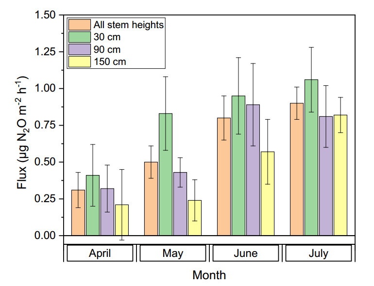
Trees growing in natural and managed environments have the capacity to act as conduits for the transport of greenhouse gases produced belowground to the atmosphere. Nitrous oxide (N₂O) emissions have been observed from tree stems in natural ecosystems but have not yet been measured in the context of forested former landfill sites. This research gap was addressed by an investigation quantifying stem and soil N₂O emissions from a closed UK landfill and a comparable natural site. Measurements were made by using flux chambers and gas chromatography over a four-month period. Analyses showed that the average N₂O stem fluxes from the landfill and non-landfill sites were 0.63 ± 0.06 μg m^–2 h^–1 and 0.26 ± 0.05 μg m^–2 h^–1, respectively. The former landfill site showed seasonal patterns in N₂O stem emissions and decreasing N₂O fluxes with increased stem sampling position above the forest floor. Tree stem emissions accounted for 1% of the total landfill N₂O surface flux, which is lower than the contribution of stem fluxes to the total surface flux in dry and flooded boreal forests.

References

[1]	Myhre G, Shindell D, Bréon FM, et al. (2013) Anthropogenic and natural radiative forcing. In: Stocker TF, Qin D, Plattner GK, et al. (eds.) Climate Change 2013: The Physical Science Basis. Contribution of Working Group Ⅰ to the Fifth Assessment Report of the Intergovernmental Panel on Climate Change. Cambridge, United Kingdom and New York, NY, USA: Cambridge University Press.
[2]	Tian H, Xu R, Canadell J, et al. (2020) A comprehensive quantification of global nitrous oxide sources and sinks. Nature 586: 248–256. https://doi.org/10.1038/s41586-020-2780-0 doi: 10.1038/s41586-020-2780-0
[3]	Ravishankara AR, Daniel JS, Portmann RW (2009) Nitrous oxide (N₂O): The dominant ozone-depleting substance emitted in the 21st century. Science 326: 123–125. https://www.science.org/doi/10.1126/science.1176985
[4]	Portmann RW, Daniel JS, Ravishankara AR (2012) Stratospheric ozone depletion due to nitrous oxide: Influences of other gases. Philos Trans R Soc B 367: 1256–1264. https://doi.org/10.1098/rstb.2011.0377 doi: 10.1098/rstb.2011.0377
[5]	Mandernack K, Kinney CA, Coleman D, et al.(2000) The biogeochemical controls of N₂O production and emission in landfill cover soils: The role of methanotrophs in the nitrogen cycle. Environ Microbiol 2: 298–309. https://doi.org/10.1046/j.1462-2920.2000.00106.x doi: 10.1046/j.1462-2920.2000.00106.x
[6]	Dìaz-Pinés E, Heras P, Gasche R, et al. (2016) Nitrous oxide emissions from stems of ash (Fraxinus angustifolia vahl) and European beech (Fagus sylvatica l.). Plant Soil 398: 35–45. https://doi.org/10.1007/s11104-015-2629-8 doi: 10.1007/s11104-015-2629-8
[7]	Smithson P, Addison, K, Atkinson K (2002) Fundamentals of the Physical Environment, London, Routledge.
[8]	Machacova, K, Papen, H, Kreuzwieser, J et al. (2013) Inundation strongly stimulates nitrous oxide emissions from stems of the upland tree Fagus sylvatica and the riparian tree Alnus glutinosa. Plant Soil 364: 287–301. https://doi.org/10.1007/s11104-012-1359-4 doi: 10.1007/s11104-012-1359-4
[9]	Moldaschl, E, Kitzler, B, Machacova, K et al. (2021) Stem CH₄ and N₂O fluxes of Fraxinus excelsior and Populus alba trees along a flooding gradient. Plant Soil 461: 407–420. https://doi.org/10.1007/s11104-020-04818-4 doi: 10.1007/s11104-020-04818-4
[10]	Machacova K, Bäck J, Vanhatalo A, et al. (2016). Pinus sylvestris as a missing source of nitrous oxide and methane in boreal forest. Nature Sci Rep 6: 23410. https://doi.org/10.1038/srep23410 doi: 10.1038/srep23410
[11]	EPA (Environmental Protection Agency) (2003) Evapotranspiration landfill cover systems fact sheet. https://clu-in.org/download/remed/epa542f03015.pdf.
[12]	Fraser-McDonald A, Boardman C, Gladding T, et al. (2022a) Methane emissions from trees planted on a closed landfill site. Waste Manage Res 40: 1618–1628. https://doi.org/10.1177/0734242X221086955 doi: 10.1177/0734242X221086955
[13]	Fraser-McDonald A, Boardman C, Gladding T, et al. (2022) Methane emissions from forested closed landfill sites: Variations between tree species and landfill management practices. Sci Total Environ 838: 156019. https://doi.org/10.1016/j.scitotenv.2022.156019 doi: 10.1016/j.scitotenv.2022.156019
[14]	Rinne J, Pihlatie M, Lohila A et al. (2005) Nitrous oxide emissions from a municipal landfill. Environ Sci Technol 39: 7790–7793. https://doi.org/10.1021/es048416q doi: 10.1021/es048416q
[15]	Zhang H, He P, Shao L (2009) N₂O emissions at municipal solid waste landfill sites: Effects of CH₄ emissions and cover soil. Atmos Environ 43: 2623–2631. https://doi.org/10.1016/j.atmosenv.2009.02.011 doi: 10.1016/j.atmosenv.2009.02.011
[16]	Börjesson G, Svensson BH (1997) Nitrous oxide emissions from landfill cover soils in Sweden. Tellus 49B: 357–363. https://doi.org/10.1034/j.1600-0889.49.issue4.2.x = doi: 10.1034/j.1600-0889.49.issue4.2.x=
[17]	Lewis E, Quinn N, Blenkinsop S, et al. (2019) Gridded estimates of hourly areal rainfall for Great Britain (1990–2014). Available: https://eip.ceh.ac.uk/data
[18]	Bollmann A, Conrad R (1998) Influence of O₂ availability on NO and N₂O release by nitrification and denitrification in soils. Global Change Bio 4: 387–396. https://doi.org/10.1046/j.1365-2486.1998.00161.x. doi: 10.1046/j.1365-2486.1998.00161.x
[19]	Wang X, Jia M, Lin X, et al. (2017) A comparison of CH₄, N₂O and CO₂ emissions from three different cover types in a municipal solid waste landfill. J Air Waste Manage 67: 507–515. https://doi.org/10.1080/10962247.2016.1268547 doi: 10.1080/10962247.2016.1268547
[20]	Skiba U (2008) 'Denitrification', in Jørgensen, S E & Fath, B D (eds.) Encyclopedia of Ecology. Elsevier B.V., 866–871. Available: https://www.sciencedirect.com/science/article/pii/B9780080454054002640?via = ihub
[21]	Bruhn D, Albert KR, Mikkelsen TN, et al. (2014). UV-induced N₂O emission from plants. Atmos Environ 99: 206–214. https://doi.org/10.1016/j.atmosenv.2014.09.077 doi: 10.1016/j.atmosenv.2014.09.077
[22]	Timilsina A, Zhang C, Pandey B, et al. (2020) Potential pathway of nitrous oxide formation in plants. Front Plant Sci 11: 1177.https://doi.org/10.3389/fpls.2020.01177 doi: 10.3389/fpls.2020.01177
[23]	Yamulki S (2017) Tree emissions of CH₄ and N₂O: Briefing and review of current knowledge Available: https://www.forestresearch.gov.uk/documents/7487/Tree_emission_of_CH4_and_N₂O_Sirwan_Yamulki_Oct2017-online.pdf.
[24]	Perämäki M, Nikinmaa E, Sevanto S, et al. (2001) Tree stem diameter variations and transpiration in Scots pine: An analysis using a dynamic sap flow model. Tree Physiol 21: 889–897. https://doi.org/10.1093/treephys/21.12-13.889 doi: 10.1093/treephys/21.12-13.889
[25]	Pihlatie M, Ambus P, Rinne J, et al. (2005) Plant-mediated nitrous oxide emissions from beech (Fagus sylvatica) leaves. New Phytol 168: 93–98. https://doi.org/10.1111/j.1469-8137.2005.01542.x doi: 10.1111/j.1469-8137.2005.01542.x

Environ-10-02-018-s001.pdf

Reader Comments

Your name:*

Email:*
© 2023 the Author(s), licensee AIMS Press. This is an open access article distributed under the terms of the Creative Commons Attribution License (http://creativecommons.org/licenses/by/4.0)