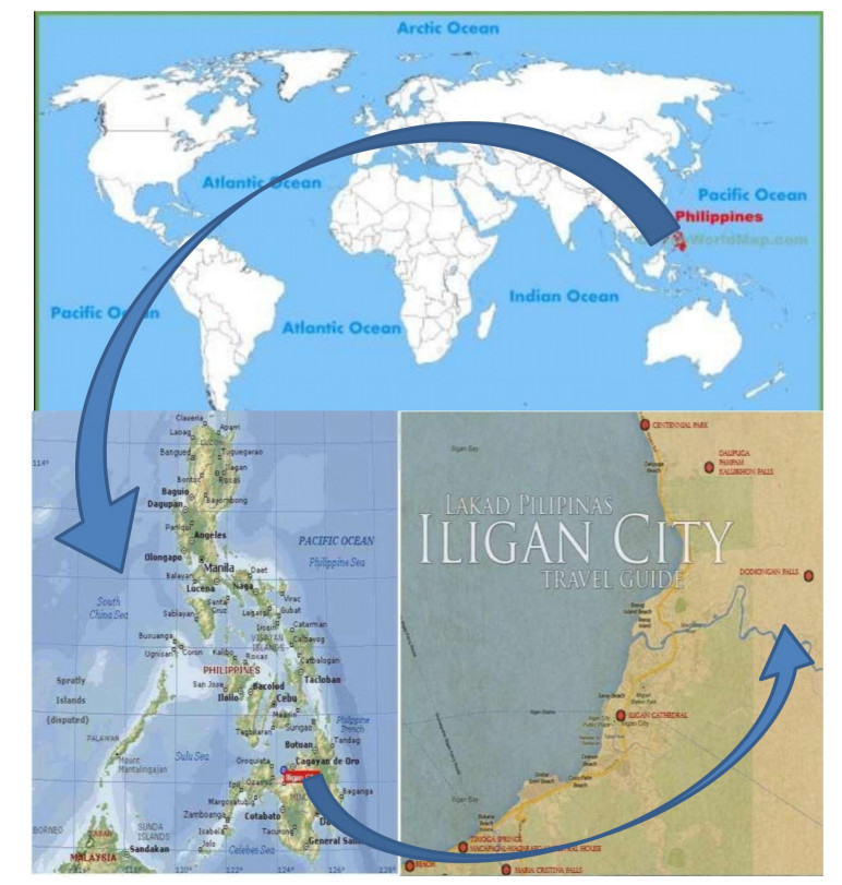
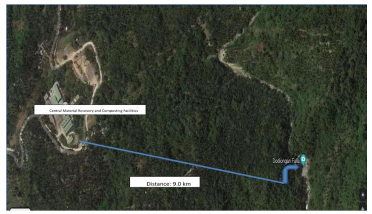
Water is an essential element that sustains life on this planet, yet it is threatened by human activities. With little attention paid to the waterfall as a source of a domestic water supply and a tourist spot for recreation, this study was designed to investigate one of the waterfalls in Iligan City, Philippines: Dodiongan Falls. The location of the study is a neighborhood of the city garbage dumpsite that due to an uncontrollable situation, releases dark-colored secretion from the treatment box as has been verified by the residents in the area; this posed a threat to their food security and livelihood. Assessing the physicochemical parameters, heavy metal concentration and Escherichia coli counts is very crucial in interpreting its water quality. All parameters such as the pH, alkalinity, turbidity, lead (Pb), mercury (Hg), and the E. Coli test were done following the standard procedures. The results revealed that the pH, alkalinity, turbidity, total lead (less than 0.01 mg/L) and total mercury concentration (less than 0.001 mg/L) at the three sites were in conformity with the guidelines of the World Health Organization and Philippine national water quality standards. However, the E. Coli count has increased downstream from 220 to 1,600 MPN per 100 ml, which exceeded the standard limit. With these findings, it is paramount that the creation of a management plan be initiated as soon as possible by the different governmental agencies in order to bring back the life of Dodiongan Falls.
Citation: Cyril A. Cabello, Nelfa D. Canini, Barbara C. Lluisma. Water quality assessment of Dodiongan Falls in Bonbonon, Iligan City, Philippines[J]. AIMS Environmental Science, 2022, 9(4): 526-537. doi: 10.3934/environsci.2022031
Water is an essential element that sustains life on this planet, yet it is threatened by human activities. With little attention paid to the waterfall as a source of a domestic water supply and a tourist spot for recreation, this study was designed to investigate one of the waterfalls in Iligan City, Philippines: Dodiongan Falls. The location of the study is a neighborhood of the city garbage dumpsite that due to an uncontrollable situation, releases dark-colored secretion from the treatment box as has been verified by the residents in the area; this posed a threat to their food security and livelihood. Assessing the physicochemical parameters, heavy metal concentration and Escherichia coli counts is very crucial in interpreting its water quality. All parameters such as the pH, alkalinity, turbidity, lead (Pb), mercury (Hg), and the E. Coli test were done following the standard procedures. The results revealed that the pH, alkalinity, turbidity, total lead (less than 0.01 mg/L) and total mercury concentration (less than 0.001 mg/L) at the three sites were in conformity with the guidelines of the World Health Organization and Philippine national water quality standards. However, the E. Coli count has increased downstream from 220 to 1,600 MPN per 100 ml, which exceeded the standard limit. With these findings, it is paramount that the creation of a management plan be initiated as soon as possible by the different governmental agencies in order to bring back the life of Dodiongan Falls.

| [1] |
Al-Badaii F, Shuhaimi-Othman M (2015) Water pollution and its impact on the prevalence of antibiotic-resistant E. coli and total coliform bacteria: a study of the Semenyih River, Peninsular Malaysia. Water Quality, Exposure and Health 7: 319–330. https://doi.org/10.1007/s12403-014-0151-5 doi: 10.1007/s12403-014-0151-5

|
| [2] |
Molina-Navarro E, Trolle D, Martínez-Pérez S, et al. (2014) Hydrological and water quality impact assessment of a Mediterranean limno-reservoir under climate change and land use management scenarios. Journal of hydrology 509: 354–366. https://doi.org/10.1016/j.jhydrol.2013.11.053 doi: 10.1016/j.jhydrol.2013.11.053
|
| [3] |
Oyekanmi FB, Bello-Olusoji OA, Akin-Obasola BJ (2017) Water quality parameters of Olumirin waterfall in relation to availability of Caridina africana (Kingsley, 1822) in Erin-Ijesa, Nigeria. Madridge J Aquac Res Dev 1: 8-12. https://doi:10.18689/mjard-1000102 doi: 10.18689/mjard-1000102
|
| [4] |
Santos EM, Mariano G, do Nascimento MAL (2015) Geotouristic potential of waterfalls in igneous and metamorphic rocks: the case of the city of bonito, Pernambuco, northeast Brazil/O potencial geoturístico de cachoeiras em rochas ígneas e metamórficas. Caderno de Geografia 25: 179-191. https://doi.org/10.5752/P.2318-2962.2015v25n43p179 doi: 10.5752/P.2318-2962.2015v25n43p179
|
| [5] |
Hanasaki N, Fujimori S, Yamamoto T, et al. (2013) A global water scarcity assessment under Shared Socio-economic Pathways–Part 2: Water availability and scarcity. Hydrology and Earth System Sciences 17: 2393-2413. https://doi.org/10.5194/hess-17-2393-2013 doi: 10.5194/hess-17-2393-2013
|
| [6] |
Amoako J, Karikari AY, Ansa-Asare OD (2011) Physico-chemical quality of boreholes in Densu Basin of Ghana. Applied Water Science 1: 41-48. https://doi.org/10.1007/s13201-011-0007-0 doi: 10.1007/s13201-011-0007-0
|
| [7] |
Arnell NW, Gosling SN (2013) The impacts of climate change on river flow regimes at the global scale. Journal of Hydrology: 486: 351-364. https://doi.org/10.1016/j.jhydrol.2013.02.010 doi: 10.1016/j.jhydrol.2013.02.010
|
| [8] | Camposano AVC, Pelone MS, Violanda R, et al. Extraction of Waterfalls from DTM using OBIA: A Case Study of Mantayupan Falls in Barili, Cebu. |
| [9] |
Offem BO, Ikpi GU (2011) Water quality and environmental impact assessment of a tropical waterfall system. Environment and Natural Resources Research 1: 63. https://doi.org/10.5539/enrr.v1n1p63 doi: 10.5539/enrr.v1n1p63
|
| [10] | Ayodele SO (2015) WATER QUALITY ASSESSMENT OF ARINTA AND OLUMIRIN WATERFALLS IN EKITI AND OSUN STATES, SOUTH WESTERN NIGERIA. International Journal of Innovative Environmental Studies Research 3:32-47. |
| [11] | Richardson SD, Kimura SY (2015) Water analysis: emerging contaminants and current issues. Analytical chemistry 88: 546-582. |
| [12] |
Kaewla W, Wiwanitkit V (2016) Accidental risk analysis in three big waterfalls in Southern Laos. Annals of Tropical Medicine and Public Health 9. https://doi.org/10.4103/1755-6783.179105 doi: 10.4103/1755-6783.179105
|
| [13] | Enguito MRC, Matunog VE, Bala JJO, et al. (2013) Water quality assessment of Carangan estero in Ozamiz City, Philippines. Journal of Multidisciplinary Studies 1. |
| [14] |
Dettori M, Pittaluga P, Busonera G, et al. (2020) Environmental risks perception among citizens living near industrial plants: a cross-sectional study. International journal of environmental research and public health 17; 4870. https://doi.org/10.3390/ijerph17134870 doi: 10.3390/ijerph17134870
|
| [15] |
Bena A, Gandini M, Cadum E, et al. (2019) Risk perception in the population living near the Turin municipal solid waste incineration plant: Survey results before start-up and communication strategies. BMC Public Health 19: 1-9. https://doi.org/10.1186/s12889-019-6808-z doi: 10.1186/s12889-019-6808-z
|
| [16] |
Liu L, Oza S, Hogan D, et al. (2016) Global, regional, and national causes of under-5 mortality in 2000–15: an updated systematic analysis with implications for the Sustainable Development Goals. The Lancet 388: 3027-3035. https://doi.org/10.1016/S0140-6736(16)31593-8 doi: 10.1016/S0140-6736(16)31593-8
|
| [17] |
Soggiu ME, Inglessis M, Gagliardi RV, et al. (2020) PM10 and PM2.5 qualitative source apportionment using selective wind direction sampling in a port-industrial area in Civitavecchia, Italy. Atmosphere 11: 94. https://doi.org/10.3390/atmos11010094 doi: 10.3390/atmos11010094
|
| [18] | Brauman KA, Siebert S, Foley JA (2013) Improvements in crop water productivity increase water sustainability and food security—a global analysis. Environmental Research Letters 8: 024030. |
| [19] |
Clayton PD, Pearson RG (2016) Harsh habitats? Waterfalls and their faunal dynamics in tropical Australia. Hydrobiologia 775: 123-137. https://doi.org/10.1007/s10750-016-2719-5 doi: 10.1007/s10750-016-2719-5
|
| [20] |
Tandang DN, Rubite RR, Angeles Jr RT, et al. (2016) Begonia titoevangelistae (sect. Baryandra, Begoniaceae) a new species from Catanduanes Island, the Philippines. Phytotaxa 282: 273-281. https://doi.org/10.11646/phytotaxa.282.4.4 doi: 10.11646/phytotaxa.282.4.4
|
| [21] |
Duan W, He B, Nover D, et al. (2016) Water quality assessment and pollution source identification of the eastern Poyang Lake Basin using multivariate statistical methods. Sustainability 8: 133. https://doi.org/10.3390/su8020133 doi: 10.3390/su8020133
|
| [22] | World Health Organization, WHO, World Health Organisation Staff (2004) Guidelines for drinking-water quality (Vol. 1). World Health Organization. |
| [23] |
Renaud FG, Le TTH, Lindener C, et al. (2015). Resilience and shifts in agro-ecosystems facing increasing sea-level rise and salinity intrusion in Ben Tre Province, Mekong Delta. Climatic Change 133: 69-84. https://doi.org/10.1007/s10584-014-1113-4 doi: 10.1007/s10584-014-1113-4
|
| [24] |
Bain R, Cronk R, Hossain R, et al. (2014) Global assessment of exposure to faecal contamination through drinking water based on a systematic review. Tropical Medicine & International Health 19: 917-927. https://doi.org/10.1111/tmi.12334 doi: 10.1111/tmi.12334
|
| [25] |
Sadat-Noori SM, Ebrahimi K, Liaghat AM (2014) Groundwater quality assessment using the Water Quality Index and GIS in Saveh-Nobaran aquifer, Iran. Environmental Earth Sciences 71: 3827-3843. https://doi.org/10.1007/s12665-013-2770-8 doi: 10.1007/s12665-013-2770-8
|
| [26] |
Altenburger R, Ait-Aissa S, Antczak P, et al. (2015) Future water quality monitoring—Adapting tools to deal with mixtures of pollutants in water resource management. Science of the total environment 512: 540-551. https://doi.org/10.1016/j.scitotenv.2014.12.057 doi: 10.1016/j.scitotenv.2014.12.057
|
| [27] |
Glassmeyer ST, Furlong ET, Kolpin DW, et al. (2017) Nationwide reconnaissance of contaminants of emerging concern in source and treated drinking waters of the United States. Science of the Total Environment 581: 909-922. https://doi.org/10.1016/j.scitotenv.2016.12.004 doi: 10.1016/j.scitotenv.2016.12.004
|
| [28] |
Islam MS, Ahmed MK, Raknuzzaman M, et al. (2015) Heavy metal pollution in surface water and sediment: a preliminary assessment of an urban river in a developing country. Ecological indicators 48: 282-291. https://doi.org/10.1016/j.ecolind.2014.08.016 doi: 10.1016/j.ecolind.2014.08.016
|
| [29] |
Ji X, Dahlgren RA, Zhang M (2016) Comparison of seven water quality assessment methods for the characterization and management of highly impaired river systems. Environmental monitoring and assessment 188: 1-16. https://doi.org/10.1007/s10661-015-5016-2 doi: 10.1007/s10661-015-5016-2
|
| [30] | Philippine National Water Quality Standards (2007) PNWQS Guidelines for Drinking Water Quality PNWQS, Philippines. |
| [31] |
Mustacisa MM, Bodiongan C, Montes V, et al. (2017). Epidemiological Study on Kawasan Waterfalls. International Journal of Environmental Science & Sustainable Development 1: 9. https://doi.org/10.21625/essd.v2i1.78 doi: 10.21625/essd.v2i1.78
|
| [32] | Su GL (2008) Assessing the effect of a dumpsite to groundwater quality in Payatas, Philippines. American Journal of Environmental Sciences 4: 276. |
Figures(3) / Tables(6)

Cyril A. Cabello, Nelfa D. Canini, Barbara C. Lluisma. Water quality assessment of Dodiongan Falls in Bonbonon, Iligan City, Philippines[J]. AIMS Environmental Science, 2022, 9(4): 526-537. doi: 10.3934/environsci.2022031


 DownLoad: