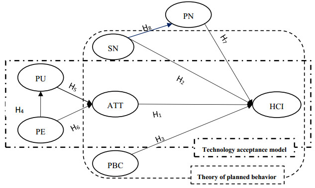
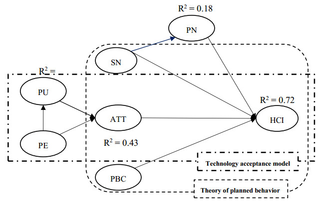
Home composting (HC) can be a cost-effective strategy for organic solid waste management. This option is also desirable since HC is increasingly automated, with HC machines composting faster than conventional composting in outdoor settings. Besides, HC may reduce organic solid waste management costs, especially for developing countries with scarcer resources. Taking Iran as a study case, the paper examines the influence of variables pertaining to the theory of planned behavior, the value-belief-norm framework, and the technology acceptance model. This study uses data collected from a territory-wide survey (n = 367) of Isfahan's residents to predict HC intentions. The results show that both attitude and subjective norms appear as the most impactful of all variables. These results further vary according to sex, with women being significantly more prone to HC than men. The findings may provide a reference to implement HC in Iran and other developing countries and possibly developed ones.
Citation: Hamid Rastegari Kopaei, Mehdi Nooripoor, Ayatollah Karami, Myriam Ertz. Modeling consumer home composting intentions for sustainable municipal organic waste management in Iran[J]. AIMS Environmental Science, 2021, 8(1): 1-17. doi: 10.3934/environsci.2021001
Home composting (HC) can be a cost-effective strategy for organic solid waste management. This option is also desirable since HC is increasingly automated, with HC machines composting faster than conventional composting in outdoor settings. Besides, HC may reduce organic solid waste management costs, especially for developing countries with scarcer resources. Taking Iran as a study case, the paper examines the influence of variables pertaining to the theory of planned behavior, the value-belief-norm framework, and the technology acceptance model. This study uses data collected from a territory-wide survey (n = 367) of Isfahan's residents to predict HC intentions. The results show that both attitude and subjective norms appear as the most impactful of all variables. These results further vary according to sex, with women being significantly more prone to HC than men. The findings may provide a reference to implement HC in Iran and other developing countries and possibly developed ones.

| [1] |
Tonglet M, Phillips PS, Bates MP (2004) Determining the drivers for householder pro-environmental behavior: Waste minimization compared to recycling. Resour Conserv Recycl 42: 27–48. doi: 10.1016/j.resconrec.2004.02.001

|
| [2] |
Abdel-Shafy HI, Mansour MSM (2018) Solid waste issue: Sources, composition, disposal, recycling, and valorization. Egypt J Pet 27: 1275–1290. doi: 10.1016/j.ejpe.2018.07.003
|
| [3] |
Price JL, Joseph JB (2000) Demand management–a basis for waste policy: a critical review of the applicability of the waste hierarchy in terms of achieving sustainable waste management. Sustain Dev 8: 96–105. doi: 10.1002/(SICI)1099-1719(200005)8:2<96::AID-SD133>3.0.CO;2-J
|
| [4] |
Mosler HJ, Tamas A, Tobias R, et al. (2008) Deriving Interventions on the Basis of Factors Influencing Behavioral Intentions for Waste Recycling, Composting, and Reuse in Cuba. Environ Behav 40: 522–544. doi: 10.1177/0013916507300114
|
| [5] |
Llatas C, Osmani M (2016) Development and validation of a building design waste reduction model. Waste Manage 56: 318–336. doi: 10.1016/j.wasman.2016.05.026
|
| [6] |
Morone P, Koutinas A, Gathergood N, et al. (2019) Food waste: Challenges and opportunities for enhancing the emerging bio-economy. J Clean Prod 221: 10–16. doi: 10.1016/j.jclepro.2019.02.258
|
| [7] |
Wang J, Li Z, Tam VWY (2015) Identifying best design strategies for construction waste minimization. J Clean Prod 92: 237–247. doi: 10.1016/j.jclepro.2014.12.076
|
| [8] |
Zorpas AA, Lasaridi K, Voukkali I, et al. (2015) Household waste compositional analysis variation from insular communities in the framework of waste prevention strategy plans. Waste Manage 38: 3–11. doi: 10.1016/j.wasman.2015.01.030
|
| [9] |
Yau Y (2012) Stakeholder engagement in waste recycling in a high-rise setting. Sustain Dev 20: 115–127. doi: 10.1002/sd.468
|
| [10] |
Meng X, Tan X, Wang Y, et al. (2019) Investigation on decision-making mechanism of residents' household solid waste classification and recycling behaviors. Resour Conserv Recycl 140: 224–234. doi: 10.1016/j.resconrec.2018.09.021
|
| [11] |
Ng SL (2019) An assessment of multi-family dwelling recycling in Hong Kong: A managerial perspective. Waste Manage 89: 294–302. doi: 10.1016/j.wasman.2019.04.014
|
| [12] |
Yang H, Zhang S, Ye W, et al. (2020) Emission reduction benefits and efficiency of e-waste recycling in China. Waste Manage 102: 541–549. doi: 10.1016/j.wasman.2019.11.016
|
| [13] |
Ertz M, Karakas F, Sarigöllü E (2016) Exploring pro-environmental behaviors of consumers: An analysis of contextual factors, attitude, and behaviors. J Bus Res 69: 3971–3980. doi: 10.1016/j.jbusres.2016.06.010
|
| [14] |
Ertz M, Durif F, Lecompte A, et al. (2018) Does "sharing" mean "socially responsible consuming"? Exploration of the relationship between collaborative consumption and socially responsible consumption. JCM 35: 392–402. doi: 10.1108/JCM-09-2016-1941
|
| [15] | Hoornweg D, Bhada-Tata P (2012) What a waste: a global review of solid waste management. Urban development series; knowledge papers, no. 15. World Bank, Washington, DC. © World Bank. |
| [16] |
Xu Z, Elomri A, Pokharel S, et al. (2017) Global reverse supply chain design for solid waste recycling under uncertainties and carbon emission constraint. Waste Manage 64: 358–370. doi: 10.1016/j.wasman.2017.02.024
|
| [17] |
Andersen MS (2007) An introductory note on the environmental economics of the circular economy. Sustain Sci 2: 133–140. doi: 10.1007/s11625-006-0013-6
|
| [18] | Shams M, Nabipour I, Dobaradaran S, et al. (2013) An environmental friendly and cheap adsorbent (municipal solid waste compost ash) with high efficiency in removal of phosphorus from aqueous solution. Fresenius Environ Bull 22. |
| [19] |
Loan LTT, Takahashi Y, Nomura H, et al. (2019) Modeling home composting behavior toward sustainable municipal organic waste management at the source in developing countries. Resour Conserv Recycl 140: 65–71. doi: 10.1016/j.resconrec.2018.08.016
|
| [20] |
Edgerton E, McKechnie J, Dunleavy K (2009) Behavioral Determinants of Household Participation in a Home Composting Scheme. Environ Behav 41: 151–169. doi: 10.1177/0013916507311900
|
| [21] |
Colón J, Martínez-Blanco J, Gabarrell X, et al. (2010) Environmental assessment of home composting. Resour Conserv Recycl 54: 893–904. doi: 10.1016/j.resconrec.2010.01.008
|
| [22] | Bartelings H, Sterner T (1999) Household Waste Management in a Swedish Municipality: Determinants of Waste Disposal, Recycling and Composting. ERE 13: 473–491. |
| [23] |
Andersen JK, Boldrin A, Christensen TH, et al. (2012) Home composting as an alternative treatment option for organic household waste in Denmark: An environmental assessment using life cycle assessment-modelling. Waste Manage 32: 31–40. doi: 10.1016/j.wasman.2011.09.014
|
| [24] |
Tanaka M (2007) Waste management for a sustainable society. Journal of Material Cycles and Waste Manage 9: 2–6. doi: 10.1007/s10163-006-0164-7
|
| [25] | Ueta K, Koizumi H (2001) Reducing Household Waste: Japan Learns from Germany. Environ Sci Policy 43: 20–32. |
| [26] | Isfahan Municipal Waste Management Organization (2019) Isfahan Municipal Waste Management Organization. Available from: http://pasmand.isfahan.ir/fa |
| [27] | Statistical Centre of Iran (2016) Statistical-Yearbook-2016-2017. Available from: https://www.amar.org.ir/english/Iran-Statistical-Yearbook/Statistical-Yearbook-2016-2017 |
| [28] | Ando A W, Gosselin A Y (2005) Recycling in Multifamily Dwellings: Does Convenience Matter? Econ Inq 43: 426–438. |
| [29] | Weinstein D, Norton C (2014) Recycling and Waste Reduction—Center for Environmental Policy and Management. Available from: https://louisville.edu/cepm/project-areas-1/recycling-and-waste-reduction |
| [30] | Foley M (2009) Indoor Composting Systems. Chowhound. Available from: https://www.chowhound.com/food-news/54730/indoor-composting-systems/ |
| [31] | McCandless SG (2010) How Indoor Automatic Composting Systems Work. HowStuffWorks. Available from: https://home.howstuffworks.com/indoor-automatic-composting-system.htm |
| [32] | Na W, Gang L, Hongming Z (2019) Design and Research of Home Automatic Kitchen Waste Composting device. In E3S Web of Conferences 136: 04013. EDP Sciences. |
| [33] | Fishbein M (1979) A theory of reasoned action: Some applications and implications. Nebr Symp Motiv 27: 65–116. |
| [34] | Fishbein M, Ajzen I (2011) Predicting and Changing Behavior: The Reasoned Action Approach (1st Ed.). Psychology Press. |
| [35] |
Chase K, Reicks M, Jones J M (2003) Applying the theory of planned behavior to promotion of whole-grain foods by dietitians. J Am Diet Assoc 103: 1639–1642. doi: 10.1016/j.jada.2003.09.026
|
| [36] |
Liou D, Bauer K (2007) Exploratory Investigation of Obesity Risk and Prevention in Chinese Americans. J Nutr Educ Behav 39: 134–141. doi: 10.1016/j.jneb.2006.07.007
|
| [37] |
Ajzen I (1991) The theory of planned behavior. Organ Behav Hum Decis Process 50: 179–211. doi: 10.1016/0749-5978(91)90020-T
|
| [38] |
Ajzen I (2002) Residual Effects of Past on Later Behavior: Habituation and Reasoned Action Perspectives. Pers Soc Psychol Rev 6: 107–122. doi: 10.1207/S15327957PSPR0602_02
|
| [39] |
Taylor S, Todd P (1997) Understanding the Determinants of Consumer Composting Behavior1. J Appl Soc Psychol 27: 602–628. doi: 10.1111/j.1559-1816.1997.tb00651.x
|
| [40] |
Thøgersen J (1999) Spillover processes in the development of a sustainable consumption pattern. J Econ Psychol 20: 53–81. doi: 10.1016/S0167-4870(98)00043-9
|
| [41] |
Barr S (2003) Strategies for sustainability: Citizens and responsible environmental behaviour. Area 35: 227–240. doi: 10.1111/1475-4762.00172
|
| [42] |
Chen MF, Tung PJ (2010) The Moderating Effect of Perceived Lack of Facilities on Consumers' Recycling Intentions. Environ Behav 42: 824–844. doi: 10.1177/0013916509352833
|
| [43] | Tucker P, Speirs D (2003) Attitudes and Behavioural Change in Household Waste Management Behaviours. J Environ Plan. Manag. 46: 289–307. |
| [44] |
Meng X, Wen Z, Qian Y (2018) Multi-agent based simulation for household solid waste recycling behavior. Resour Conserv Recycl 128: 535–545. doi: 10.1016/j.resconrec.2016.09.033
|
| [45] |
Valle POD, Rebelo E, Reis E, et al. (2005) Combining Behavioral Theories to Predict Recycling Involvement. Environ Behav 37: 364–396. doi: 10.1177/0013916504272563
|
| [46] |
Knussen C, Yule F, MacKenzie J, et al. (2004) An analysis of intentions to recycle household waste: The roles of past behaviour, perceived habit, and perceived lack of facilities. J Environ Psychol 24: 237–246. doi: 10.1016/j.jenvp.2003.12.001
|
| [47] |
Kim TG, Lee JH, Law R (2008) An empirical examination of the acceptance behaviour of hotel front office systems: An extended technology acceptance model. Tour Manag 29: 500–513. doi: 10.1016/j.tourman.2007.05.016
|
| [48] | Benbasat I, Barki H (2007) Quo vadis TAM? J Assoc Inf Syst 8: 211–218. |
| [49] | Saade R, Kira D (2006) The Emotional State of Technology Acceptance. ⅡSIT 3: 529–539. |
| [50] |
Broman TM, Schuitema G, Thøgersen J (2014) Responsible technology acceptance: Model development and application to consumer acceptance of Smart Grid technology. Appl Energy 134: 392–400. doi: 10.1016/j.apenergy.2014.08.048
|
| [51] |
Davies J, Foxall GR, Pallister J (2002) Beyond the Intention–Behaviour Mythology. Mark Theory 2: 29–113. doi: 10.1177/1470593102002001645
|
| [52] |
Bamberg S, Moser G M (2007) Twenty years after Hines, Hungerford, and Tomera: A new meta-analysis of psycho-social determinants of pro-environmental behaviour. J Environ Psychol 27: 14–25. doi: 10.1016/j.jenvp.2006.12.002
|
| [53] |
Zeweld W, Van Huylenbroeck G, Tesfay G, et al. (2017) Smallholder farmers' behavioural intentions towards sustainable agricultural practices. J Environ Manage 187: 71–81. doi: 10.1016/j.jenvman.2016.11.014
|
| [54] |
Yuan Y, Nomura H, Takahashi Y, et al. (2016) Model of Chinese Household Kitchen Waste Separation Behavior: A Case Study in Beijing City. Sustainability 8: 1083–1083. doi: 10.3390/su8101083
|
| [55] |
Bamberg S, Hunecke M, Blöbaum A (2007) Social context, personal norms and the use of public transportation: Two field studies. J Environ Psychol 27: 190–203. doi: 10.1016/j.jenvp.2007.04.001
|
| [56] | Byun J, Jang S (2019) Can signaling impact customer satisfaction and behavioral intentions in times of service failure? Evidence from open versus closed kitchen restaurants. J Hosp Mark Manag 28: 785–806. |
| [57] |
Onwezen MC, Antonides G, Bartels J (2013) The Norm Activation Model: An exploration of the functions of anticipated pride and guilt in pro-environmental behaviour. J Econ Psychol 39: 141–153. doi: 10.1016/j.joep.2013.07.005
|
| [58] |
Park J, Ha S (2014) Understanding Consumer Recycling Behavior: Combining the Theory of Planned Behavior and the Norm Activation Model. Fam Consum Sci Res J 42: 278–291. doi: 10.1111/fcsr.12061
|
| [59] |
Han H, Hwang J, Lee M J, et al. (2019) Word-of-mouth, buying, and sacrifice intentions for eco-cruises: Exploring the function of norm activation and value-attitude-behavior. Tour Manag 70: 430–443. doi: 10.1016/j.tourman.2018.09.006
|
| [60] |
Liao C, Zhao D, Zhang S, et al. (2018) Determinants and the moderating effect of perceived policy effectiveness on residents' separation intention for rural household solid waste. Int J Environ Res Public Health 15: 726. doi: 10.3390/ijerph15040726
|
| [61] |
Oztekin C, Teksöz G, Pamuk S, et al. (2017) Gender perspective on the factors predicting recycling behavior: Implications from the theory of planned behavior. Waste Manage 62: 290–302. doi: 10.1016/j.wasman.2016.12.036
|
| [62] |
Zhou Y, Zhou Q, Gan S, et al. (2018) Factors affecting farmers' willingness to pay for adopting vegetable residue compost in North China. Acta Ecologica Sinica 38: 401–411. doi: 10.1016/j.chnaes.2018.04.001
|
| [63] | Pedhazur EJ (1997) Multiple Regression in Behavioral Research: Explanation and Prediction, 3rd Ed. New York: Holt, Rinehart and Winston, 1997. (p. 1058). Wadsworth. |
| [64] |
Chu PY, Chiu J (2003) Factors Influencing Household Waste Recycling Behavior: Test of an Integrated Model. J Appl Soc Psychol 33: 604–626. doi: 10.1111/j.1559-1816.2003.tb01915.x
|
| [65] | Miles J, Shevlin M (2001) Applying Regression and Correlation: A Guide for Students and Researchers (First edition). SAGE Publications Ltd. |
| [66] | Hair JF, Hult GTM, Ringle C M, et al. (2017) Mirror, mirror on the wall: A comparative evaluation of composite-based structural equation modeling methods. J Acad Mark. 45: 616–632. |
| [67] |
Fornell C, Larcker DF (1981) Structural Equation Models with Unobservable Variables and Measurement Error: Algebra and Statistics. J Mark Res 18: 382–388. doi: 10.1177/002224378101800313
|
| [68] |
Tenenhaus M, Vinzi V E, Chatelin Y-M, et al. (2005) PLS path modeling. Comput Stat Data An, 48: 159–205. doi: 10.1016/j.csda.2004.03.005
|
| [69] | Ipsos (2018) Global views on the environment–2018. Available from: https://www.ipsos.com/sites/default/files/Global_Views_on_the_Environment.pdf (accessed on 17-02-2020). |
| [70] |
Stern PC (2000) New Environmental Theories: Toward a Coherent Theory of Environmentally Significant Behavior. J Soc Issues 56: 407–424. https://doi.org/10.1111/0022-4537.00175 doi: 10.1111/0022-4537.00175
|
| [71] |
de Leeuw A, Valois P, Ajzen I, et al. (2015) Using the theory of planned behavior to identify key beliefs underlying pro-environmental behavior in high-school students: Implications for educational interventions. J Environ Psychol 42: 128–138. doi: 10.1016/j.jenvp.2015.03.005
|
| [72] |
Ertz M, Huang R, Jo MS, et al. (2017) From single-use to multi-use: Study of consumers' behavior toward consumption of reusable containers. J Environ Manage 193: 334–344. doi: 10.1016/j.jenvman.2017.01.060
|
| [73] | Dutta S, Bhaskar S (2018) Bengaluru's All Women Trio Teaches Composting Via WhatsApp To Learners Across The World | Women's Day. NDTV-Dettol Banega Swasth Swachh India. Available from: https://swachhindia.ndtv.com/bengalurus-all-women-trio-teaches-composting-via-whatsapp-to-learners-across-the-world-17788/ |
| [74] | CCAP (2015) Tackling waste through community-based composting – Bangladesh. Available from: https://ccap.org/assets/CCAP-Booklet_BangladeshCompost.pdf (accessed on 17-02-2020). |
| [75] | Sutta S, Bhaskar S (2018) Bengaluru's All Women Trio Teaches Composting via WhatsApp to Learners across the World. Available from: https://swachhindia.ndtv.com/bengalurus-all-women-trio-teaches-composting-via-whatsapp-to-learners-across-the-world-17788/ (accessed on 17-02-2020). |
| [76] | Pearson AR, Ballew MT, Naiman S, et al. (2017) Race, Class, Gender and Climate Change Communication. Oxford Research Encyclopedia of Climate Science Available from: https://doi.org/10.1093/acrefore/9780190228620.013.412 |
| [77] | Ballew M, Marlon J, Leiserowitz A, et al. (2018) Gender Differences in Public Understanding of Climate Change. Yale Program on Climate Change Communication. Available from: https://climatecommunication.yale.edu/publications/gender-differences-in-public-understanding-of-climate-change/ |
 Environ-08-01-01-S1.pdf Environ-08-01-01-S1.pdf |
 |
Figures(2) / Tables(4)

Hamid Rastegari Kopaei, Mehdi Nooripoor, Ayatollah Karami, Myriam Ertz. Modeling consumer home composting intentions for sustainable municipal organic waste management in Iran[J]. AIMS Environmental Science, 2021, 8(1): 1-17. doi: 10.3934/environsci.2021001


 DownLoad: