
Citation: Vanessa Duarte Pinto, Catarina Martins, José Rodrigues, Manuela Pires Rosa. Improving access to greenspaces in the Mediterranean city of Faro[J]. AIMS Environmental Science, 2020, 7(3): 226-246. doi: 10.3934/environsci.2020014
[1] | Bandar Abdullah Aloyaydi, Subbarayan Sivasankaran, Hany Rizk Ammar . Influence of infill density on microstructure and flexural behavior of 3D printed PLA thermoplastic parts processed by fusion deposition modeling. AIMS Materials Science, 2019, 6(6): 1033-1048. doi: 10.3934/matersci.2019.6.1033 |
[2] | K.A. Lazopoulos, A.K. Lazopoulos . Beam bending and Λ-fractional analysis. AIMS Materials Science, 2023, 10(4): 604-617. doi: 10.3934/matersci.2023034 |
[3] | Guadalupe Sanchez-Olivares, Fausto Calderas, Antonio Sanchez-Solis, Luis Medina-Torres, Leonardo R. Moreno, Octavio Manero . Assessment of extrusion-sonication process on flame retardant polypropylene by rheological characterization. AIMS Materials Science, 2016, 3(2): 620-633. doi: 10.3934/matersci.2016.2.620 |
[4] | Marek Konieczny . Mechanical properties and failure analysis of laminated magnesium-intermetallic composites. AIMS Materials Science, 2022, 9(4): 572-583. doi: 10.3934/matersci.2022034 |
[5] | Kiyotaka Obunai, Daisuke Mikami, Tadao Fukuta, Koichi Ozaki . Microstructure and mechanical properties of newly developed SiC-C/C composites under atmospheric conditions. AIMS Materials Science, 2018, 5(3): 494-507. doi: 10.3934/matersci.2018.3.494 |
[6] | R. Daulath Banu, R. Karunanithi, S. Sivasankaran, B. Subramanian, Abdullah A. Alhomidan . Influence of graphene nanoplatelets (GNPs) and aluminum-carbon layered double hydroxides (Al-C LDH) in polypropylene matrix of hybrid composite structures on the microstructure and mechanical performances. AIMS Materials Science, 2024, 11(5): 882-917. doi: 10.3934/matersci.2024043 |
[7] | Mohammed O. Atteaa Al-hassany, Ali Al-Dulaimy, Amir Al-Sammarraie, Abed Fares Ali . Effect of fiberglass form on the tensile and bending characteristic of epoxy composite material. AIMS Materials Science, 2020, 7(5): 583-595. doi: 10.3934/matersci.2020.5.583 |
[8] | Hanh C. Nguyen, Shigeru Nagasawa, Kensei Kaneko . Strength estimation of silicon nitride ceramics using a round-notched specimen subjected to shearing-tool indentation. AIMS Materials Science, 2020, 7(5): 518-533. doi: 10.3934/matersci.2020.5.518 |
[9] | Bhavik Ardeshana, Umang Jani, Ajay Patel, Anand Joshi . An approach to modelling and simulation of single-walled carbon nanocones for sensing applications. AIMS Materials Science, 2017, 4(4): 1010-1028. doi: 10.3934/matersci.2017.4.1010 |
[10] | Zulzamri Salleh, Md Mainul Islam, Jayantha Ananda Epaarachchi, Haibin Su . Mechanical properties of sandwich composite made of syntactic foam core and GFRP skins. AIMS Materials Science, 2016, 3(4): 1704-1727. doi: 10.3934/matersci.2016.4.1704 |
Brain tumors are abnormal cell growths located in or near brain tissue that damage the nervous system, causing symptoms such as headaches, dizziness, dementia, seizures, and other neurological signs [1]. Magnetic resonance imaging (MRI)—including T1-weighted (T1), post-contrast T1-weighted (T1CE), T2-weighted (T2), and fluid-attenuated inversion recovery (FLAIR) sequences—is a prevalent diagnostic tool for brain tumors due to its sensitivity to soft tissue and high image contrast, as shown in Figure 1. Physicians utilize MRI for lesion diagnosis, but accuracy can be hindered by factors such as fatigue and emotional state. Automated methods have garnered extensive attention in the medical field due to their capability to objectively and accurately analyze imaging information.
Most multimodal approaches assume complete data availability; however, in reality, missing modalities are common. As illustrated in Figure 2, various missing scenarios can occur during both training and inference stages. The absence of certain MRI sequences may fail to capture tumor characteristics, thereby limiting a comprehensive understanding of the tumor [2]. Therefore, it is crucial for multimodal learning methods to maintain robustness in the presence of missing modalities during inference.
Currently, a prevalent approach to tackle segmentation arising from missing modality is knowledge distillation [3,4], where information is transferred from a teacher-student network to recover missing data, but this can be computationally intensive. Another method is image synthesis [5], leveraging generative models to reconstruct the missing data. However, synthetic images may introduce noise to the task. Additionally, mapping available modalities into a common latent subspace aims to compensate for or recover the missing information [6,7,8]. However, existing approaches often require training multiple sets of parameters to address various missing modality scenarios, thereby escalating the model's complexity and computational overhead.
With the expansion of data scale and enhancement of computational resources, researchers favor general neural networks for diverse tasks, minimizing the need for task-specific model design and training. Recently, transformer [9] has shown great potential in natural language processing, visual recognition, intensive prediction. However, its complex architecture and high computational demands limit comprehensive fine-tuning for downstream tasks, especially accurate segmentation, potentially leading to overfitting and reduced generalization ability.
Inspired by recent advancements in prompt learning [10,11,12] and efficient fine-tuning techniques [13,14,15], we introduce a novel brain tumor segmentation framework, called DPONet. This framework employs an encoder-decoder structure for the segmentation network, enhancing performance in both incomplete and complete modality scenarios. Specifically, we leverage image frequency information as frequency filtering prompt (FFP) to facilitate the pre-trained model in extracting discriminative features. Furthermore, by learning a series of spatial perturbation prompt (SPP), we map these discriminative features into a common latent space, mitigating the challenges of modality fusion in the decoder. Finally, we validate the robustness of our approach on two commonly used public datasets. To sum up, our main contributions are as follows:
● We propose a new framework for incomplete-modal image segmentation that effectively handles common cases of missing modalities. This approach requires only 7% of the trainable parameters to adjust the pre-trained model, thereby avoiding the heavy fine-tuning typically necessary for transformers.
● We introduce a frequency filtering prompt to extract spatial frequency components from images. This method addresses the model's oversight of target domain features and enhances its adaptation to brain tumor datasets.
● We propose a spatial perturbation prompt that incorporates learnable parameters into a spatial modulation model. This aims to achieve consistent multimodal feature embeddings even in the presence of missing partial modalities.
Incomplete multimodal learning refers to scenarios in multimodal learning tasks where partial modality information is missing or incomplete. This issue becomes particularly prominent in brain tumor segmentation tasks, where medical imaging data is typically composed of multiple MRI sequences. The absence of one modality results in the challenge of incomplete modality information learning. Many studies [16,17,18] are devoted to solving this problem, demonstrating impressive performance in various incomplete multimodal learning tasks. Zhou et al. [16] showed that there exists a certain correlation within the latent representations of modalities, which can be utilized to describe missing modalities by calculating the correlation between modalities in a latent space. Ting et al. [17] combines available modality information to estimate the latent features of missing modalities. Liu et al. [18] explicitly considers the relationship between modalities and regions, giving different attention to different modalities for each region. However, these models require full fine-tuning of the pre-trained model, which increases the computational burden and leads to a decrease in generalization ability.
The task of most neural networks is to learn the optimal points in functions. Fourier Transform establishes the transformation relationship between the function in the spatial domain and the frequency domain, so that we can analyze a function by the frequency component to approximate the objective function more effectively [19]. The frequency of an image represents the intensity of gray change in the image. Fourier transform analyzes the features by analyzing the coefficients of each frequency component [20]. The performance of computer vision models is significantly affected by the Fourier statistical properties of the training data and show a certain sensitivity to the Fourier basis direction, and their robustness can be improved by learning this sensitivity [21]. For example, Fang et al. [22] and Xu et al. [23] argued that different parts of the same organ in MRI images exhibit regularity and that high-frequency structural information can more effectively capture these similarities and regularities.
Prompt learning is an effective transfer learning approach in natural language processing [10,24,25], which fine-tunes pre-trained models on source tasks by embedding contextual prompts. Recently, prompts have also been employed in computer vision tasks [26,27,28] and multimodal learning tasks [11,29,30], introducing self-adaptation in the input space to optimize the target task. For instance, Jia et al. [26] proposed the Pyramid Vision Transformer model (PVT), achieving downstream performance comparable to full fine-tuning by adding a small number of learnable prompt embeddings on the patch embedding. Different from the PVT model, Bahng et al. [27] further proposed a method to learn a single disturbance to adjust the pixel space and affect the model output. These studies suggest that continuously adjusting and optimizing prompts can enhance the adaptability of model. Lee et al. [29] treats different scenarios of missing modalities as different types of inputs and employs learnable prompts to guide the predictions of model under various missing conditions. Qiu et al. [30] utilizes an intermediate classifier to generate a prompt for each missing scenario based on intermediate features for segmentation prediction. The difference is that our work does not require learning a set of prompts for each missing scenario but aims to learn generic visual prompts and generalize them to modulate feature space in missing scenes.
In this paper, we focus on brain tumor segmentation under common missing modality scenarios. We simulate real-world data incompleteness by assuming absences of one or multiple modalities (Figure 2). Additionally, due to the difficulty of fully training a pre-trained transformer with limited computational resources, we design a discriminative prompt optimization network that avoids fine-tuning the entire pre-trained model. In this section, we will elaborate on the framework and its components.
The pyramid vision transformer (PVT) [31] introduces a progressive shrinking strategy within the transformer block to control the scale of feature maps for dense prediction tasks. We chose the backbone is initialized with the weights pre-trained on ImageNet. PVT comprises four stages, each consisting of a patch embedding layer and l transformer encoder layers, which generate feature maps of different scales. Given an input image X∈RH×W×C, the patch embedding layer divides the sample X into HWpi non-overlapping patches, where pi represents the patch size of the i-th layer. As the stage progresses, the patch size decreases accordingly. The flattened patches are then fed into a linear projection to obtain embedded patches. The embedded patches, along with positional embedding information, are subsequently input into the transformer encoder to produce a feature map x of size Hpi×Wpi×C.This process can be described as follows:
xl=MLP(LN(SRA(xl−1))), | (3.1) |
where xl−1 represents the feature map output from the previous layer, SRA(⋅) denotes the spatial reduction attention proposed in PVT, and LN(⋅) and MLP(⋅) refer to normalization and multi-layer perceptron operations, respectively. SRA is like multi-head attention. The formula is as follows:
SQA=Attention(QWQ,SRA(K)WK,SR(V)WV), | (3.2) |
where WQ, WK, and WV are the parameters of the linear projections. SRA(⋅) is used to reduce the spatial dimension. This can be expressed as:
SRA(x)=LN(Reshape(xi,ri)WS), | (3.3) |
The ri represents the feature map reduction rate for stage i.
The Reshape(⋅) operation reshapes the input x∈Rhi×wi×ci to hiwir2i×(r2ici)). The WS is a linear projection that reduces the dimensionality of the input. The attention calculation is as follows:
Attention(q,k,v)=Softmax(qkT√d)v, | (3.4) |
where q, k and v are the query, key, and value transform matrices, and d is the dimension.
We consider a multimodal dataset consisting of N(N=4) modalities, M= FLAIR, T1CE, T1 and T2. The dataset is denoted as D=D14,D13,…,Di,…,D0, where D14 represents the complete set of modalities, and other sets represent missing modalities subsets, such as D0=XF0,XT1c0,XT10,XT21 indicating only T2 mode is available. Xmk represents the input sample, where m denotes the modality type, and k represents the modal state. For the model, it is unaware of which specific modality is missing, therefore, we introduce placeholder values (set to 0) to assign to the missing modality data XF0,XT1c0,XT10,XT20 to ensure the format of the multimodal input.
We propose a novel discriminative prompt optimization network, as shown in Figure 3, which aims to provide natural insertion points for intermediate features of the network while preserving the integrity of the pre-trained model and enabling fine-tuning for downstream tasks. We adapt a pre-trained transformer as feature extractor and keep it frozen during training. Multimodal images D={Xkm}k=[0,1] are fed into four extractors, and task-relevant information is aggregated through discriminative prompts to fully exploiting the discriminative features. Next, a spatial perturbation prompt module is introduced, which hierarchically fuses the discriminative features of available modalities and maps them to a shared feature representation space to learn cross-modal shared information. Furthermore, the fused features are mapped back to the original input size through up-sampling in the decoder, and the resulting segmentation masks are obtained from these feature maps. Notably, during training, the trainable parameters are confined to the prompt components and the decoder.
The frequency filtering prompt method, as illustrated in Figure 4, utilizes Fourier transform to extract frequency features and jointly modulates the intermediate features with image embeddings. The frequency processing method decomposes images into different frequency components, which are distributed across different spatial locations of the image, encouraging the model to focus on critical information of the image [21]. The core idea is to remodulate the intermediate features using frequency domain information, shifting the distribution from the pre-trained dataset to the target dataset. Furthermore, since there may be commonalities between features of different modalities, even if image data from a particular modality is missing, the remaining modalities still contain corresponding frequency information, which enhances the robustness of the information to a certain extent. Taking a single branch as an example, for a given image, we apply the fast Fourier transform (FFT) along the spatial dimension to obtain frequency components corresponding to different spatial locations. FFT is applied to each channel to convert the spatial domain representation into a frequency representation in the frequency domain, and filtering operations are performed in the frequency domain. Then, an attention mask is learned in the frequency domain to analyze the dominant frequency components in the feature map. Finally, the feature representation is transformed back to the spatial domain using inverse FFT (iFFT). The transformation from the spatial domain to the frequency domain is expressed as follows:
F(x)(μ,υ)=H−1∑h=0W−1∑w=0x(h,w)e−i2π(hμH+wυW), | (3.5) |
After obtaining the frequency representation, different frequency components are modulated by filtering through the attention mechanism. Specifically, the attention mechanism compresses information across channels through convolution and a sigmoid function. The expression of the frequency filtering mechanism is as follows:
F′(x)=Fx⊗σ(conv([AvgPool(Fx),Maxpool(Fx)])), | (3.6) |
where, σdenotes the Sigmoid function, AvgPool(⋅) and MaxPool(⋅) represent the average pooling and max pooling operations respectively.
Finally, the inverse FFT is used to transform back to the spatial domain features:
x′(h,w)=1H⋅WH−1∑h=0W−1∑w=0F′(x)ei2π(hμH+wυW), | (3.7) |
Inspired by AdaptFormer [32], we employ a frequency enhancement adaptor, a bottleneck structure that limits the number of parameters. It takes the combination of filtered frequency features and image features as input and generates relevant frequency prompts through a down-projection layer, a lightweight multi-layer perceptron, and an up-projection layer. Formally, this process can be expressed as:
pif=MLPup(GELU(MLPidown(x′+x))), | (3.8) |
Thirdly, the generated prompts are appended to the transformer layers to facilitate the model in learning more representative and discriminative image features.
To enable the model to handle missing modalities, we employ null values for filling, however, such null values are likely to disturb the feature space and result in failure of modal feature fusion. Therefore, we propose learnable spatial perturbation prompts, as show in Figure 5, aiming to learn a task-specific visual prompt (P) within a latent space that encourages the sharing of cross-modal information. Prompts interact dynamically with input features, facilitating adaptive modal fusion rather than simply injecting fixed information using learning prompts.
First, the extracted discriminative features are concatenated through element-wise addition fic=[fif,fit1c,fit1,fit2] and then passed through a 3 × 3 convolutional layer followed by a Sigmoid activation function to generate prompt weights ωi∈[0,1]. These weights describe the importance of each spatial data point in the input. Inspired by EVP [27], we add random visual embeddings of the same size as the transformer tokens, train only these random embeddings in the training phase, and the trained visual prompts as the guidance for the model, denoted as Fi=(Fitoken,pim). The process can be described as:
ωi=σ(conv([fif,fit1c,fit1,fit2])), | (3.9) |
pim=conv(N∑c=1ωipic), | (3.10) |
Fi=transformer(fic+pim), | (3.11) |
where, σ is the Sigmoid function. Finally, the cross-modal information features (F) are fed into Transformer encoder block to establish cross-modal long-range dependencies.
We introduce a consistency loss to optimize the prompts to capture task-shared knowledge and transform it into representations that are beneficial for the task. Specifically, we map the feature maps obtained from the transformer encoder stages to the same size as the input image and use mean squared error ensuring that the model learns coherent and consistent information at each stage. Note that, since shallower layers may lack sufficient semantic information, we apply the consistency loss only in the last two stages of the transformer encoder.
Lm=1NN∑i=1M∑m=1(ˆfi−fmi)2, | (3.12) |
where, N is the number of samples, M is the number of decoder layers, and the rescaled features of images in transformer layer m, and their average is denoted as ˆfi=1m∑mk=1fki.
In addition, we mapped the feature map into a segmentation map, and calculated Dice loss from the ground truth to prompt the model capture consistent feature representations.
Ld=1NN∑i=1M∑m=1Dice(yi−f(xim)), | (3.13) |
where, yi denotes the ground-truth labels of the image xi, and f(xim) denotes the prediction corresponding to the m-th layer features of the image.
The feature consistency loss and prediction consistency loss are combined to supervise prompt generation.
Lc=γLm+(1−γ)Ld, | (3.14) |
where, γ is the weight parameter used to balance the two losses. We experiment with different values of γ and found that γ=0.3 gives the best result.
The convolutional decoder gradually restores the spatial resolution from the fused features to the original segmentation space. The convolutional decoder employs skip connections to merge features from different modalities at specific hierarchical levels into the encoder, to preserve more low-level details. Therefore, the overall processing steps are as follows:
Di=conv(upsample(conv(fic,Di−1))), | (3.15) |
where Di is the feature map from the i-th layer of the convolutional decoder, and fic is the combined feature from multiple encoder layers.
We employ a hybrid loss to measure the difference between the predictions and the ground truth. Dice Loss is used to calculate the similarity between the predicted segmentation result and the true segmentation result. Cross-entropy loss measures the prediction performance by quantifying the difference between the predicted probability distribution and the true probability distribution. Gradients are calculated based on the feedback of the sum of the two losses to update the parameters. The definition is as follows:
LDice=−2∑Niyif(xi)∑Niyi+∑Nif(xi), | (3.16) |
LCE=−∑Niyilogp(f(xi)), | (3.17) |
where f(xi) and yi represent the prediction and ground-truth labels, respectively. Besides, N is the number of pixels, p(⋅) is the SoftMax of the prediction. Last, our hybid loss function Lseg can be given by
Lseg=Lc+LDice+LCE, | (3.18) |
We use two public datasets from the Multimodal Brain Tumor Segmentation Challenge (BraTS) to demonstrate the effectiveness of the proposed method, BraTS 2018 and BraTS 2020 [33,34,35]. BraTS 2018 contains 285 cases of patients for training, while BraTS 2020 includes 369 cases for training and 125 for validation. In these datasets, each case comprises four MRI modalities: Flair, T1ce, T1, and T2. The volume of each modality is 240 × 240 × 155, aligned within the same spatial space. Medical experts provide manual pixel-level annotations of three mutually inclusive tumor regions in each image, namely, whole tumor (WT), tumor core (TC), and enhancing tumor (ET). WT encompasses all tumor tissues, while TC comprises ET, necrosis, and non-enhancing tumor core.
Data preprocessing is performed on the two datasets before training. For each dataset, we slice along the axial plane of the 3D medical images. To eliminate non-informative slices and irrelevant background regions, thereby saving training efficiency and time, we use central slices as the training data and reshape each 2D slice to 224 × 224. We design a simulation method for missing modalities. The MRI modalities are randomly removed from the input. The missing modality can be any one or multiple modalities, and the missing rate for each modality is random. The purpose of this is to simulate the scenario where missing modalities may occur in real-world situations.
In this study, our method is implemented in Pytorch utilizing a single NVIDIA Tesla V100 32 GB GPU. We adopt the U-Net architecture composed of transformer blocks as the benchmark, and the transformer is pre-trained on ImageNet-1K. We utilize the SGD optimizer with an initial learning rate of 0.01. After many experiments and parameter tuning, we set our model to train 100 epochs with an initial learning rate of 1e−2 and a batch size of 12. For the segmentation task, we use the Dice coefficient (which computes the similarity of two sets), the Hausdorff distance (HD95, which measures the distance between two sets), and the sensitivity (the ratio of the number of positive samples correctly identified by the model to the number of all true positive samples) as performance metrics to evaluate various methods.
We focus on exploring the robustness of discriminative optimization networks to general incompleteness in multimodal image without fine-tuning the entire pretraind model. In this chapter, we first introduce the excellent results obtained by our method. Subsequently, a series of ablation experiments on the proposed components. Considering that the BraTS 2020 dataset contains many patient cases and is representative, we experimented with it in the ablation study.
As shown in Table 1, our method achieves remarkable performance in Dice score on both the modality-complete and modality-missing scenarios. For example, our proposed approach has significantly better mean Dice scores for whole tumors, tumor cores, and enhanced tumors than suboptimal approaches. From the experimental results in Table 2, we observed that the baseline model generally exhibited unsatisfactory performance on the T1 modality. However, our model achieved significant improvements in this aspect, effectively enhancing the performance under the T1 modality. In Figures 6 and 7, we present the visualization of segmentation results. Furthermore, Table 3 clearly exhibits that our method outperforms other approaches in terms of HD95 and sensitivity under complete modality testing, further validating the superior performance of our approach.
Modalities | Dice (%) ↑ | |||||||||||||||||
Complete | Core | Enhancing | ||||||||||||||||
F | T1 | T1c | T2 | D | Z | T | Q | Our | D | Z | T | Q | Our | D | Z | T | Q | Our |
✓ | 86.1 | 86.1 | 86.5 | 86.7 | 93.9 | 71.0 | 70.9 | 71.5 | 71.0 | 93.3 | 46.3 | 46.3 | 45.6 | 47.2 | 76.1 | |||
✓ | 76.8 | 78.5 | 77.4 | 79.5 | 91.6 | 81.5 | 84.0 | 83.4 | 84.3 | 95.3 | 74.9 | 80.1 | 78.9 | 81.4 | 88.4 | |||
✓ | 77.2 | 78.0 | 78.1 | 79.5 | 89.1 | 66.0 | 65.9 | 66.8 | 67.7 | 91.9 | 37.3 | 38.0 | 41.3 | 39.1 | 71.6 | |||
✓ | 87.3 | 87.4 | 89.1 | 86.9 | 95.2 | 69.2 | 68.8 | 69.3 | 69.9 | 93.5 | 38.2 | 42.4 | 43.6 | 42.8 | 74.6 | |||
✓ | ✓ | 87.7 | 87.8 | 88.4 | 88.4 | 94.5 | 83.5 | 84.8 | 86.4 | 86.3 | 95.8 | 75.9 | 79.4 | 81.7 | 80.1 | 88.9 | ||
✓ | ✓ | 81.1 | 81.8 | 81.2 | 83.1 | 92.1 | 83.4 | 83.6 | 85.2 | 85.8 | 95.4 | 78.0 | 80.1 | 79.2 | 81.7 | 88.3 | ||
✓ | ✓ | 89.7 | 89.8 | 89.9 | 89.8 | 95.5 | 73.1 | 73.8 | 73.9 | 74.4 | 94.3 | 41.0 | 45.9 | 48.2 | 46.8 | 77.3 | ||
✓ | ✓ | 87.7 | 87.8 | 88.0 | 87.9 | 94.4 | 73.1 | 73.4 | 73.3 | 72.9 | 94.1 | 45.7 | 46.8 | 50.1 | 47.3 | 77.5 | ||
✓ | ✓ | 89.9 | 89.9 | 90.5 | 90.1 | 95.5 | 74.1 | 74.6 | 75.5 | 74.5 | 94.1 | 49.3 | 48.6 | 48.6 | 49.5 | 76.6 | ||
✓ | ✓ | 89.9 | 89.3 | 90.0 | 90.0 | 95.6 | 84.7 | 84.8 | 85.5 | 86.6 | 95.9 | 76.7 | 81.9 | 81.8 | 81.2 | 88.9 | ||
✓ | ✓ | ✓ | 90.7 | 90.1 | 90.7 | 90.6 | 95.6 | 85.1 | 85.2 | 86.5 | 86.7 | 95.8 | 76.8 | 82.1 | 81.8 | 81.8 | 88.8 | |
✓ | ✓ | ✓ | 90.6 | 90.6 | 90.3 | 90.6 | 95.7 | 75.2 | 75.6 | 75.9 | 75.8 | 94.7 | 49.9 | 50.3 | 52.5 | 51.1 | 78.0 | |
✓ | ✓ | ✓ | 90.7 | 90.4 | 90.6 | 90.8 | 95.8 | 85.0 | 85.3 | 86.4 | 86.4 | 96.0 | 77.1 | 78.7 | 81.0 | 80.0 | 88.9 | |
✓ | ✓ | ✓ | 88.3 | 88.2 | 88.7 | 88.9 | 94.6 | 83.5 | 84.2 | 86.5 | 86.5 | 95.8 | 77.0 | 79.3 | 78.5 | 82.1 | 88.9 | |
✓ | ✓ | ✓ | ✓ | 91.1 | 90.6 | 90.6 | 91.0 | 95.9 | 85.2 | 84.6 | 87.4 | 86.4 | 95.9 | 78.0 | 79.9 | 81.6 | 81.0 | 88.9 |
Average | 87.0 | 87.1 | 87.3 | 87.6 | 94.3 | 78.2 | 78.6 | 79.6 | 79.7 | 94.8 | 61.5 | 64.0 | 64.9 | 64.9 | 82.8 |
Modalities | Dice (%) ↑ | |||||||||||||||||
Complete | Core | Enhancing | ||||||||||||||||
F | T1 | T1c | T2 | Z | Y | T | L | Our | Z | Y | T | L | Our | Z | Y | T | L | Our |
✓ | 81.2 | 76.3 | 86.6 | 84.8 | 94.3 | 64.2 | 56.7 | 68.8 | 69.4 | 94.4 | 43.1 | 16.0 | 41.4 | 47.6 | 76.2 | |||
✓ | 72.2 | 42.8 | 77.8 | 75.8 | 92.6 | 75.4 | 65.1 | 81.5 | 82.9 | 95.4 | 72.6 | 66.3 | 75.7 | 73.7 | 89.2 | |||
✓ | 67.5 | 15.5 | 78.7 | 74.4 | 90.9 | 56.6 | 16.8 | 65.6 | 66.1 | 93.2 | 32.5 | 8.1 | 44.5 | 37.1 | 74.7 | |||
✓ | 86.1 | 84.2 | 88.4 | 88.7 | 95.2 | 61.2 | 47.3 | 66.7 | 66.4 | 94.2 | 39.3 | 8.1 | 40.5 | 35.6 | 74.8 | |||
✓ | ✓ | 83.0 | 84.1 | 88.2 | 86.3 | 95.0 | 78.6 | 80.3 | 84.8 | 84.2 | 96.1 | 74.5 | 68.7 | 77.7 | 75.3 | 90.0 | ||
✓ | ✓ | 74.4 | 62.1 | 81.8 | 77.2 | 93.1 | 78.6 | 78.2 | 83.5 | 83.4 | 95.7 | 74.0 | 70.7 | 77.1 | 74.7 | 89.5 | ||
✓ | ✓ | 87.1 | 87.3 | 89.7 | 89.0 | 95.6 | 65.9 | 61.6 | 72.0 | 70.8 | 95.2 | 43.0 | 9.5 | 44.4 | 41.2 | 77.9 | ||
✓ | ✓ | 82.2 | 84.2 | 88.4 | 88.7 | 94.9 | 61.2 | 47.3 | 66.7 | 66.4 | 95.1 | 45.0 | 16.5 | 47.7 | 48.7 | 77.7 | ||
✓ | ✓ | 87.6 | 87.9 | 90.3 | 89.9 | 95.9 | 69.8 | 62.6 | 71.8 | 70.9 | 95.1 | 47.5 | 17.4 | 48.3 | 45.4 | 78.1 | ||
✓ | ✓ | 87.1 | 87.5 | 89.5 | 89.7 | 95.6 | 77.9 | 80.8 | 84.8 | 84.4 | 96.1 | 75.1 | 64.8 | 76.8 | 75.0 | 90.0 | ||
✓ | ✓ | ✓ | 87.3 | 87.7 | 90.4 | 88.9 | 95.7 | 79.8 | 80.9 | 85.2 | 84.1 | 96.2 | 75.5 | 65.7 | 77.4 | 74.0 | 90.0 | |
✓ | ✓ | ✓ | 87.8 | 88.4 | 89.7 | 89.9 | 96.0 | 71.5 | 63.7 | 74.1 | 72.7 | 95.5 | 47.7 | 19.4 | 50.0 | 44.8 | 78.7 | |
✓ | ✓ | ✓ | 88.1 | 88.8 | 90.6 | 90.4 | 96.0 | 79.6 | 80.7 | 85.8 | 84.6 | 96.3 | 75.7 | 66.4 | 76.6 | 73.8 | 90.1 | |
✓ | ✓ | ✓ | 82.7 | 80.9 | 88.4 | 86.1 | 95.1 | 80.4 | 79.0 | 85.8 | 84.4 | 96.2 | 74.8 | 68.3 | 78.5 | 75.4 | 90.1 | |
✓ | ✓ | ✓ | ✓ | 89.6 | 88.8 | 90.6 | 90.1 | 96.1 | 85.8 | 80.1 | 85.9 | 84.5 | 96.3 | 77.6 | 68.4 | 80.4 | 75.5 | 90.0 |
Average | 82.9 | 76.4 | 87.3 | 86.0 | 94.8 | 72.4 | 65.4 | 77.5 | 77.0 | 95.4 | 59.9 | 42.3 | 62.5 | 59.9 | 83.8 |
Method | Dice ↑ | HD95 ↓ | Sensitivity ↑ | |||||||||
WT | TC | ET | Avg | WT | TC | ET | Avg | WT | TC | ET | Avg | |
Ding et al. | 86.13 | 71.93 | 58.98 | 72.35 | - | - | - | - | - | - | - | - |
Zhang et al. | 87.08 | 78.69 | 64.08 | 76.62 | 2.90 | 6.21 | 44.64 | 17.92 | 99.60 | 99.81 | 99.82 | 99.74 |
Ting et al. | 90.71 | 84.60 | 79.07 | 84.79 | 4.05 | 5.78 | 33.77 | 14.53 | 90.98 | 83.90 | 77.68 | 84.18 |
Qiu et al. | 87.58 | 79.67 | 64.87 | 77.37 | 2.82 | 5.71 | 43.92 | 17.48 | 99.66 | 99.83 | 99.81 | 99.77 |
baseline(fine-tune) | 77.63 | 78.94 | 70.85 | 93.56 | 2.61 | 2.09 | 2.39 | 2.36 | 86.28 | 86.50 | 82.74 | 85.17 |
baseline(frozen) | 58.11 | 61.09 | 40.88 | 89.16 | 2.83 | 2.29 | 2.97 | 2.70 | 81.41 | 84.68 | 85.90 | 84.00 |
our | 94.96 | 94.12 | 89.98 | 93.02 | 2.58 | 2.09 | 2.21 | 2.29 | 96.81 | 96.32 | 93.01 | 95.38 |
We further conducted experiments to analyze the robustness of our proposed method to varying missing modality rates between the training and testing phases. As shown in Figure 8(a), we trained the model with a 70% missing rate and randomly removed multiple modalities to simulate modality missing scenarios for testing. We found that, compared to the baseline, our DPONet method was robust to different missing rates during testing. Moreover, in Figure 8(b), where we used 10%, 70%, and 90% to represent the degree of missingness during training (through many experiments, we found that these missing rates are representative), we observed that when training with more complete modality data, the performance was significantly higher when testing with low missing rates. In this paper, the experiments based on the general reality that collecting complete modality data cannot be guaranteed. However, there are still some publicly available datasets with complete modalities. Therefore, we trained the models using complete data, as shown in Figure 8(c), where the baseline model could not handle data missing, our method consistently improved upon the baseline.
We explored the effects of frequency filtering prompts and spatial perturbation prompts, the results showing in Table 4, our method achieved a higher Dice score of 93.02. The term baseline (fine-tune) refers to a pre-trained transformer that is comprehensively fine-tuned on the BraTS dataset. The term baseline (frozen) refers to a baseline model where the pre-trained backbone parameters are frozen.
Method | Dice ↑ | HD95 ↓ | Sensitivity ↑ | |||||||||
WT | TC | ET | Avg | WT | TC | ET | Avg | WT | TC | ET | Avg | |
baseline (fine-tune) | 77.63 | 78.94 | 70.85 | 75.81 | 2.61 | 2.09 | 2.39 | 2.36 | 86.28 | 86.50 | 82.74 | 85.17 |
baseline (frozen) | 58.11 | 61.09 | 40.88 | 53.36 | 2.83 | 2.29 | 2.97 | 2.70 | 81.41 | 84.68 | 85.90 | 84.00 |
baseline + FFP | 93.65 | 92.40 | 85.08 | 90.38 | 2.45 | 2.04 | 2.16 | 2.22 | 96.54 | 96.11 | 91.26 | 94.64 |
baseline + SPP | 94.56 | 94.40 | 87.37 | 92.11 | 2.47 | 2.05 | 2.22 | 2.25 | 96.59 | 96.07 | 90.53 | 94.40 |
baseline + FFP + SPP | 94.96 | 94.12 | 89.98 | 93.02 | 2.58 | 2.09 | 2.21 | 2.29 | 96.81 | 96.32 | 93.01 | 95.38 |
We introduced frequency filtering prompts into the baseline model, the model achieved comparable performance to fine-tuned model, demonstrating the efficiency of proposed component. Furthermore, as shown in Figure 9, during training with complete modalities, when a significant portion of modalities were absent during inference (i.e., retaining only one modality), the baseline model suffered a severe performance degradation. Excitingly, when prompts were introduced, the model was able to perform image segmentation normally even with a single modality input, indicating that the proposed visual prompts facilitated the encoder to learn discriminative features across modalities.
We introduced the spatial perturbation prompts module into the baseline, the overall robustness of the model was improved. As shown in Table 4, our method achieved a higher Dice score of 93.02, exceeding the baseline model by 17.21. Furthermore, the Dice score for the ET region saw a significant increase, indicating that the spatial perturbation prompt facilitated the fusion of inter-modal information and preserved more edge details and small-scale information. Figure 10 visualizes the segmentation results before and after using the spatial perturbation prompt, clearly demonstrating that more small-scale lesion areas are preserved.
Additionally, in Table 5, we described the parameter information before and after adding the module. It indicates that our method only introduced approximately 7% of the total trainable parameters but achieved excellent segmentation performance. Once extended to large models with billions of parameters, our proposed method will be more favorable and suitable for multimodal downstream tasks with missing modalities, achieving a favorable trade-off between computational cost and performance.
Method | Param (M) | Tunable Param (M) |
baseline (fine-tune) | 194.82 | 194.82 |
baseline (frozen) | 194.82 | 49.30 |
baseline + FFP | 160.42 | 58.97 |
baseline + SPP | 173.93 | 48.69 |
baseline + FFP + SPP | 153.43 | 10.58 |
In this paper, we introduce a parameter-efficient and discriminatively optimized segmentation network that exhibits robust adaptability to generalized missing modality inputs. Our model filters frequency features to generate discriminative visual cues and introduces learnable spatial perturbation prompts into shared feature representations, effectively addressing the challenge of incomplete multimodal brain tumor segmentation. Compared to fine-tuning the entire transformer model, our approach requires only 7% of the trainable parameters while demonstrating superior performance in handling real-world scenarios with missing modality data. Extensive experiments and ablation studies on the publicly available BraTS2018 and BraTS2020 datasets validate the effectiveness of our proposed method.
In this work, we investigate a parametrically efficient incomplete modal image segmentation method for brain tumors. Although our model successfully captures consistent features by mapping robust multimodal features to the same potential space, we must point out that our model cannot recover information about missing modalites from available multimodal inputs. Therefore, our next plan will study how to use the available multimodal image to estimate the missing modal information to obtain rich image information.
This work is supported by the National Nature Science Foundation of China (No.U24A20231, No.62272283), New Twentieth Items of Universities in Jinan (No.2021GXRC049).
All authors declare no conflicts of interest in this paper.
[1] | UN General Assembly. Transforming our world: From 2030 Agenda for Sustainable Development, 2015. Available from: https://www.refworld.org/docid/57b6e3e44.html. |
[2] | World Health Organization (2016) Urban green spaces and health, a review of evidence. Copenhagen: WHO regional office for Europe. |
[3] | European Communities (2000) Towards a local sustainability profile: European common indicators. In: Towards an urban atlas, Technical Report, Directorate-General for Environment, Luxembourg, European Commission. |
[4] | Cavaco C, Vilares E, Rosa F, et al. (2015) The Portuguese Strategy for Sustainable Cities towards smarter urban development. GEOSPATIAL World Forum: Workshop Measuring Progress Achieving Smarter Cities. Available from: http://www.unece.org/fileadmin/DAM/hlm/prgm/urbandevt/Measuring_Progress__Achieving_Smarter_Cities_/Presentations/Cristina_Cavaco.pdf. |
[5] | Fisher B, Costanza R, Turner K, et al. (2007) Defining and classifying ecosystem services for decision making. CSERGE, University of East Anglia, Norwich 07-04. |
[6] | Millennium Ecosystem Assessment (2005) Ecosystems and Human Well-being: Synthesis. In: Island Press, Washington DC. |
[7] |
Escobedo FJ, Varela S, Zhao M, et al. (2010) Analysing the efficacy of subtropical urban forests in offsetting carbon emissions from cities. Environ Sci Policy 13: 362-372. doi: 10.1016/j.envsci.2010.03.009
![]() |
[8] |
Gill S, Handley J, Ennos A, et al. (2007) Adapting cities for climate change: the role of the green infrastructure. Built Environ 33: 115-133. doi: 10.2148/benv.33.1.115
![]() |
[9] | Simpson JR, McPherson EG (1996) Potential of tree shade for reducing residential energy use in California. J Arboricult 22: 10-18. |
[10] |
Comber A, Brunsdon C, Green E (2008) Using a GIS-based network analysis to determine urban greenspace accessibility for different ethnic and religious groups. Landsc Urban Plan 86: 103-114. doi: 10.1016/j.landurbplan.2008.01.002
![]() |
[11] | Handley J, Pauleit S, Slinn P, et al. (2003) Providing accessible natural greenspace in towns and cities: a practical guide to assessing the resource and implementing local standards for provision. Centre for Urban and Regional Ecology 1-36. |
[12] | Maidstone Borough Council: Green and blue infrastructure strategy, 2016. Available from: http://www.maidstone.gov.uk/__data/assets/pdf_file/0004/164659/Green-and-Blue-Infrastructure-trategy-June-2016.pdf. |
[13] |
Bowler DE, Buyung-Ali LM, Knight TM, et al. (2010) A systematic review of evidence for the added benefits to health of exposure to natural environments. BMC Public Health 10: 456. doi: 10.1186/1471-2458-10-456
![]() |
[14] | Thompson K, Coon JB, Stein K, et al. (2011) Does participating in physical activity in outdoor natural environments have a greater effect on physical and mental wellbeing than physical activity indoors? A systematic review. Environ Sc. Technol 45: 1761-1772. |
[15] | de Vries S, Verheij R, Groenewegen P, et al. (2003) Natural environments-healthy environments? An exploratory analysis of the relationship between greenspace and health. Environ Plan A 35: 1717-173. |
[16] |
Fuller R, Irvine K, Devine-Wright P, et al. (2007) Psychological benefits of greenspace increase with biodiversity. Biol Lett 3: 390-394. doi: 10.1098/rsbl.2007.0149
![]() |
[17] |
Owen N, Healy GN, Matthews CE, et al. (2010) Too much sitting: the population-health science of sedentary behavior. Exerc Sport Sci Rev 38: 105-113. doi: 10.1097/JES.0b013e3181e373a2
![]() |
[18] |
Li Q, Morimoto K, Kobayashi M (2008) Visiting a forest, but not a city, increases human natural killer activity and expression of anti-cancer proteins. Int J Immunopath Ph 21: 117-127. doi: 10.1177/039463200802100113
![]() |
[19] | Kuo M (2015) How might contact with nature promote human health? Promising mechanisms and a possible central pathway. Front Psych 25: 1093. |
[20] |
Madureira H., Nunes F., Oliveira JV, et al. (2015) Urban residents' beliefs concerning green space benefits in four cities in France and Portugal. Urban Forest Urban Green 14: 56-64. doi: 10.1016/j.ufug.2014.11.008
![]() |
[21] | Sunyer J, Ballester F, Le Tetre A, et al. (2003) The association of daily sulfur dioxide air pollution levels with hospital admissions for cardiovascular diseases in Europe (The Aphea-II study). Eur Heart J 24 (8): 752-760. |
[22] | Bernstein JA, Alexis N, Barnes C, et al. (2004) Health effects of air pollution. J Allergy Clin Inmun 114 (5): 1116-1123. |
[23] |
Kim J, Kaplan R (2004) Physical and psychological factors in sense of community: new urbanist kentlands and nearby orchard village. Environ Behav 36: 313-340. doi: 10.1177/0013916503260236
![]() |
[24] |
Seeland K, Dubendorfer S, Hansmann R (2009) Making friends in Zurich's urban forests and parks: The role of public green space for social inclusion of youths from different cultures. Forest Policy Econ 11: 10-17. doi: 10.1016/j.forpol.2008.07.005
![]() |
[25] |
Mitchell R, Popham F (2008) Effect of exposure to natural environment on health inequalities: an observational population study. Lancet 372: 1655-1660. doi: 10.1016/S0140-6736(08)61689-X
![]() |
[26] |
Brown SC, Perrino T, Lombard J, et al. (2018) Health disparities in the relationship of neighborhood greenness to mental health outcomes in 249,405 U.S. Medicare beneficiaries. Int J Environ Res Public Health 15: 430. doi: 10.3390/ijerph15030430
![]() |
[27] |
James P, Banay RF, Hart JE, et al. (2015) A Review of the Health Benefits of Greenness. Curr Epidemiol Rep 2:131-142. doi: 10.1007/s40471-015-0043-7
![]() |
[28] |
van den Berg M, Wendel-Vos W, van Poppel M, et al. (2015) Health benefits of green spaces in the living environment: A systematic review of epidemiological studies. Urban Forest Urban Green 14: 806-816. doi: 10.1016/j.ufug.2015.07.008
![]() |
[29] |
Twohig-Bennett C, Jones A (2018) The health benefits of the great outdoors: A systematic review and meta-analysis of greenspace exposure and health outcomes. Environ Res 166: 628-637. doi: 10.1016/j.envres.2018.06.030
![]() |
[30] | Forsyth A, Musacchio L, Fitzgerald F (2005) Designing small parks: a manual for addressing social and ecological concerns, In: John Wiley & Sons, New Jersey. |
[31] |
Berardi U, GhaffarianHoseini A, GhaffarianHoseini A (2014) State-of-the-art analysis of the environmental benefits of green roofs. Appl Energy 115: 411-428. doi: 10.1016/j.apenergy.2013.10.047
![]() |
[32] |
Emilsson T (2008) Vegetation development on extensive vegetated green roofs: influence of substrate composition, establishment method and species mix. Ecol Eng 33: 265-77. doi: 10.1016/j.ecoleng.2008.05.005
![]() |
[33] | Liu K, Baskaran B (2003) Thermal performance of green roofs through field evaluation. Proceedings of the First North American Green Roof Infrastructure Conference, Chicago, USA, May 29-30, 1-10. |
[34] |
GhaffarianHoseini A, Dahlan N, Berardi U, et al. (2013) Sustainable energy performances of green buildings: a review of current theories, implementations and challenges. Renew Sustainable Energy Rev 25: 1-17. doi: 10.1016/j.rser.2013.01.010
![]() |
[35] |
Weng Q, Lu D, Schubring J (2004) Estimation of land surface temperature-vegetation abundance relationship for urban heat island studies. Remote Sens Environ 89: 467-83. doi: 10.1016/j.rse.2003.11.005
![]() |
[36] |
Bates A, Sadler J, Mackay R (2013) Vegetation development over four years on two green roofs in the UK. Urban Forest Urban Green 12: 98-108. doi: 10.1016/j.ufug.2012.12.003
![]() |
[37] | Baumann N (2006) Ground-nesting birds on green roofs in Switzerland: Preliminary observations. Urban Habitats 4 (1): 37-50. |
[38] | Colla SR, Willis E, Packer L (2009) Can green roofs provide habitat for urban bees (Hymenoptera: Apidae)? CATE 2:1-12. |
[39] |
MacIvor S, Lundholm J (2011) Insect species composition and diversity on intensive green roofs and adjacent level-ground habitats. Urban Ecosyst 14: 225-241. doi: 10.1007/s11252-010-0149-0
![]() |
[40] |
Kim KG (2004) The application of the biosphere reserve concept to urban areas: the case for green rooftops for habitat network in Seoul. Ann NY Acad Sci 1023: 187-214. doi: 10.1196/annals.1319.010
![]() |
[41] |
Ignatieva M, Stewart G, Meurk C (2011) Planning and design of ecological networks in urban areas. Landscape Ecol Eng 7: 17-25. doi: 10.1007/s11355-010-0143-y
![]() |
[42] |
Baldock K, Goddard M, Hicks D, et al. (2019) A systems approach reveals urban pollinator hotspots and conservation opportunities. Nat Ecol Evol 3: 363-373. doi: 10.1038/s41559-018-0769-y
![]() |
[43] |
Whittinghill L, Rowe D, Cregg B (2013) Evaluation of vegetable production on extensive green roofs. Agroecol Sust Food 37: 465-484. doi: 10.1080/21683565.2012.756847
![]() |
[44] | Dubbeling M, Renting H, Hoekstra F, et al. (2015) City Region Food Systems. Urban Agr Mag 29: 1-72. |
[45] |
Mears M, Brindley P (2019) Measuring Urban Greenspace Distribution Equity: The Importance of Appropriate Methodological Approaches. Int J Geo-Inf 8: 286. doi: 10.3390/ijgi8060286
![]() |
[46] | VTPI, Accessibility evaluating peoples to reach desired goods, services and activities: From TDM Encyclopedia, Victoria Transport Policy Institute, 2017. Available from: http://www.vtpi.org/tdm/tdm84.htm. |
[47] | Litman T (2017) Accessibility for transportation planning: Measuring people's ability to reach desired goods and activitie. TDM Encyclopedia, Victoria Transport Policy Institute. |
[48] | Barton H, Davis G, Guise R (1995) Sustainable Settlements-a guide for planners, designers and developers, In: Bristol University of the West of England and The Local Government Management Board. |
[49] |
Rioux L, Werner C, Mokounkolo R, et al. (2016) Walking in two French neighbourhoods: A study of how park numbers and locations relate to everyday walking. J Environ Psychol 48: 169-184. doi: 10.1016/j.jenvp.2016.10.003
![]() |
[50] |
Dai D (2011) Racial/ethnic and socioeconomic disparities in urban green space accessibility: Where to intervene? Landsc Urban Plan 102: 234-244. doi: 10.1016/j.landurbplan.2011.05.002
![]() |
[51] | Astell-Burt T, Feng X, Mavoa S, et al. (2014) Do low-income neighbourhoods have the least green space? A cross-sectional study of Australia's most populous cities. BMC Public Health 14: 292. |
[52] |
Heckert M (2013) Access and equity in greenspace provision: A comparison of methods to assess the impacts of greening vacant land. Trans GIS 17: 808-827. doi: 10.1111/tgis.12000
![]() |
[53] |
Shen Y, Sun F, Che Y (2017) Public green spaces and human wellbeing: Mapping the spatial inequity and mismatching status of public green space in the Central City of Shanghai. Urban Forest Urban Green 27: 59-68. doi: 10.1016/j.ufug.2017.06.018
![]() |
[54] | Calthorpe P (1994) Shokokusya: The Next American Metropolis-Ecology, Community and the American Dream, In: Architectural Press, Princeton. |
[55] | European Environment Agency (2002). Towards an urban atlas: Assessment of spatial data on 25 European cities and urban areas. In: Environmental issue report No 30/2002, Copenhagen. |
[56] |
van Herzele A, Wiedemann T (2003) A monitoring tool for the provision of accessible and attractive urban green spaces. Landsc Urban Plan 63: 109-126. doi: 10.1016/S0169-2046(02)00192-5
![]() |
[57] | Natural England: From 'Nature Nearby' Accessible Natural Greenspace Guidance, 2010. Available from: http://www.ukmaburbanforum.co.uk/docunents/other/nature_nearby.pdf. |
[58] | Barbosa O, Tratalos J, Armsworth P, et al. (2007) Who benefits from access to green space? A case study from Sheffield, UK. Landsc Urban Plan 83: 187-195. |
[59] |
Higgs G, Fry R, Langford M (2012) Investigating the implications of using alternative GIS-based techniques to measure accessibility to green space. Environ Plann B: Planning and Design 39: 326-343. doi: 10.1068/b37130
![]() |
[60] |
Comber A, Brunsdon C, Green E (2008) Using a GIS-based network analysis to determine urban greenspace accessibility for different ethnic and religious groups. Landsc Urban 86: 103-114. doi: 10.1016/j.landurbplan.2008.01.002
![]() |
[61] |
Li L, Du Q, Ren F, et al. (2019) Assessing Spatial Accessibility to Hierarchical Urban Parks by Multi-Types of Travel Distance in Shenzhen, China. Int. J Environ Res Public Health 16: 1038. doi: 10.3390/ijerph16061038
![]() |
[62] |
Herman K, Sbarcea M, Panagopoulos T (2018) Creating Green Space Sustainability through Low-Budget and Upcycling Strategies. Sustainability 10: 1857. doi: 10.3390/su10061857
![]() |
[63] | Instituto Nacional de Estatística (INE): From Base Geográfica de Referenciação da Informação, 2011. Available from: http://mapas.ine.pt/download/index2011.phtml. |
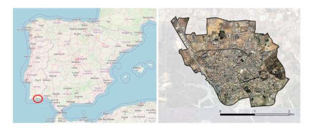
[64] | Figure 1 from: Map data copyrighted OpenStreetMap contributors. Available from: https://www.openstreetmap.org. |
[65] | Alves R, Bento R, Ramos L, et al. (2015) Integração dos usos do solo e transportes em cidades de média dimensão (InLUT). In: Relatório final, Universidade de Trás-os-Montes e Alto douro, Faculdade de Arquitectura da Universidade técnica de Lisboa e Universidade do Algarve. |
[66] | Rosa MP, Martins C, Rodrigues J (2017) The development of indicators of sustainable mobility associated with an urbanism of proximity. The Case of the City of Faro. In: INCREaSE, Proceedings of the International Congress on Engineering and Sustainability, Faro, Portugal, Springer 47-66. |
[67] |
Berte E, Panagopoulos T (2014) Enhancing city resilience to climate change by means of ecosystem services improvement: A SWOT analysis for the city of Faro, Portugal. Int J Urban Sust Dev 6: 241-253. doi: 10.1080/19463138.2014.953536
![]() |
[68] | Santos A, Terremoto R, Brito J, et al. (2008) Plano Verde de Faro-Princípios, Objectivos e Conteúdo. Câmara Municipal de Faro e Gabinete de Apoio Técnico de Faro. |
[69] | Guimarães ET, Bragança L, Almeida MG, et al. (2015) Analysis of Portuguese Residential Building and Proposed Solutions, Connecting People and Ideas. In: Proceedings of EURO ELECS, Guimarães, Portugal. |
[70] | Noocity: Urban Ecology. Available from: https://www.noocity.com/pt-pt/#. |
[71] | Huang R, Hawley D (2009) A data model and internet GIS framework for safe routes to school. URISA J 21: 21-30. |
[72] | Salvo G, Sabatini S (2014) Advanced or and AI methods in transportation a Gis approach to evaluate bus stop accessibility. Available from: http://www.iasi.cnr.it/ewgt/16conference/ID108.pdf. |
[73] | Scheurer J, Curtis C (2007) Accessibility measures: Overview and practical applications. Urbanet Department of Urban and Regional Planning, Curtin University. |
[74] | Geurs K, Ritsema van Eck J (2001) Accessibility measures: review and applications, evaluation of accessibility impacts of land-use transport scenarios and related social and economic impacts. Rese Man Environ 408505 006. |
[75] | Achuthan K, Titheridge H, Mackett RL (2007) Measuring pedestrian accessibility. In: Winstanley, Proceedings of the Geographical Information Science Research, National University of Ireland, Maynooth, UK, vol. 11-13, 264-269. |
[76] |
Bhatti M, Church A (2004) Home the culture of nature and meanings of gardens in late modernity. Housing Studies 19: 37-51. doi: 10.1080/0267303042000152168
![]() |
[77] |
Coolen H, Meesters J (2012) Private and public green spaces: meaningful but different settings. J Hous Built Environ 27:49-67. doi: 10.1007/s10901-011-9246-5
![]() |
[78] | Boumeester HJFM, Dol K., Meesters J (2009) Stedelijk wonen: een brug tussen wens en werkelijkheid. Een onderzoek naar woonwensen en woonproducten bij binnenstedelijk bouwen (Urban living: bridging preferences and reality. Housing preference and housing products for urban development). Voorburg: NVB. |
[79] | Bernardini C, Irvine KN (2007) The 'nature' of urban sustainability: private or public green spaces. In: A. Kungolas, C. A. Brebbia, & E. Beriatos, (Eds.), Sustainable development and planning III, volume 2, WIT Press: 661-674. |
[80] |
Russo A, Cirella G (2018) Modern Compact Cities: How Much Greenery Do We Need? Int J Environ Res Public Health 15: 2180. doi: 10.3390/ijerph15102180
![]() |
[81] |
Oliver LN, Schuurman N, Hall AW (2007) Comparing circular and network buffers to examine the influence of land use on walking for leisure and errands. Int J Health Geograph 6: 41. doi: 10.1186/1476-072X-6-41
![]() |
[82] | Lyytimäki J, Petersen LK, Normander B, et al. (2008) Nature as a nuisance? Ecosystem services and disservices to urban lifestyle. J Environ Sci 5 (3): 161-172. |
Modalities | Dice (%) ↑ | |||||||||||||||||
Complete | Core | Enhancing | ||||||||||||||||
F | T1 | T1c | T2 | D | Z | T | Q | Our | D | Z | T | Q | Our | D | Z | T | Q | Our |
✓ | 86.1 | 86.1 | 86.5 | 86.7 | 93.9 | 71.0 | 70.9 | 71.5 | 71.0 | 93.3 | 46.3 | 46.3 | 45.6 | 47.2 | 76.1 | |||
✓ | 76.8 | 78.5 | 77.4 | 79.5 | 91.6 | 81.5 | 84.0 | 83.4 | 84.3 | 95.3 | 74.9 | 80.1 | 78.9 | 81.4 | 88.4 | |||
✓ | 77.2 | 78.0 | 78.1 | 79.5 | 89.1 | 66.0 | 65.9 | 66.8 | 67.7 | 91.9 | 37.3 | 38.0 | 41.3 | 39.1 | 71.6 | |||
✓ | 87.3 | 87.4 | 89.1 | 86.9 | 95.2 | 69.2 | 68.8 | 69.3 | 69.9 | 93.5 | 38.2 | 42.4 | 43.6 | 42.8 | 74.6 | |||
✓ | ✓ | 87.7 | 87.8 | 88.4 | 88.4 | 94.5 | 83.5 | 84.8 | 86.4 | 86.3 | 95.8 | 75.9 | 79.4 | 81.7 | 80.1 | 88.9 | ||
✓ | ✓ | 81.1 | 81.8 | 81.2 | 83.1 | 92.1 | 83.4 | 83.6 | 85.2 | 85.8 | 95.4 | 78.0 | 80.1 | 79.2 | 81.7 | 88.3 | ||
✓ | ✓ | 89.7 | 89.8 | 89.9 | 89.8 | 95.5 | 73.1 | 73.8 | 73.9 | 74.4 | 94.3 | 41.0 | 45.9 | 48.2 | 46.8 | 77.3 | ||
✓ | ✓ | 87.7 | 87.8 | 88.0 | 87.9 | 94.4 | 73.1 | 73.4 | 73.3 | 72.9 | 94.1 | 45.7 | 46.8 | 50.1 | 47.3 | 77.5 | ||
✓ | ✓ | 89.9 | 89.9 | 90.5 | 90.1 | 95.5 | 74.1 | 74.6 | 75.5 | 74.5 | 94.1 | 49.3 | 48.6 | 48.6 | 49.5 | 76.6 | ||
✓ | ✓ | 89.9 | 89.3 | 90.0 | 90.0 | 95.6 | 84.7 | 84.8 | 85.5 | 86.6 | 95.9 | 76.7 | 81.9 | 81.8 | 81.2 | 88.9 | ||
✓ | ✓ | ✓ | 90.7 | 90.1 | 90.7 | 90.6 | 95.6 | 85.1 | 85.2 | 86.5 | 86.7 | 95.8 | 76.8 | 82.1 | 81.8 | 81.8 | 88.8 | |
✓ | ✓ | ✓ | 90.6 | 90.6 | 90.3 | 90.6 | 95.7 | 75.2 | 75.6 | 75.9 | 75.8 | 94.7 | 49.9 | 50.3 | 52.5 | 51.1 | 78.0 | |
✓ | ✓ | ✓ | 90.7 | 90.4 | 90.6 | 90.8 | 95.8 | 85.0 | 85.3 | 86.4 | 86.4 | 96.0 | 77.1 | 78.7 | 81.0 | 80.0 | 88.9 | |
✓ | ✓ | ✓ | 88.3 | 88.2 | 88.7 | 88.9 | 94.6 | 83.5 | 84.2 | 86.5 | 86.5 | 95.8 | 77.0 | 79.3 | 78.5 | 82.1 | 88.9 | |
✓ | ✓ | ✓ | ✓ | 91.1 | 90.6 | 90.6 | 91.0 | 95.9 | 85.2 | 84.6 | 87.4 | 86.4 | 95.9 | 78.0 | 79.9 | 81.6 | 81.0 | 88.9 |
Average | 87.0 | 87.1 | 87.3 | 87.6 | 94.3 | 78.2 | 78.6 | 79.6 | 79.7 | 94.8 | 61.5 | 64.0 | 64.9 | 64.9 | 82.8 |
Modalities | Dice (%) ↑ | |||||||||||||||||
Complete | Core | Enhancing | ||||||||||||||||
F | T1 | T1c | T2 | Z | Y | T | L | Our | Z | Y | T | L | Our | Z | Y | T | L | Our |
✓ | 81.2 | 76.3 | 86.6 | 84.8 | 94.3 | 64.2 | 56.7 | 68.8 | 69.4 | 94.4 | 43.1 | 16.0 | 41.4 | 47.6 | 76.2 | |||
✓ | 72.2 | 42.8 | 77.8 | 75.8 | 92.6 | 75.4 | 65.1 | 81.5 | 82.9 | 95.4 | 72.6 | 66.3 | 75.7 | 73.7 | 89.2 | |||
✓ | 67.5 | 15.5 | 78.7 | 74.4 | 90.9 | 56.6 | 16.8 | 65.6 | 66.1 | 93.2 | 32.5 | 8.1 | 44.5 | 37.1 | 74.7 | |||
✓ | 86.1 | 84.2 | 88.4 | 88.7 | 95.2 | 61.2 | 47.3 | 66.7 | 66.4 | 94.2 | 39.3 | 8.1 | 40.5 | 35.6 | 74.8 | |||
✓ | ✓ | 83.0 | 84.1 | 88.2 | 86.3 | 95.0 | 78.6 | 80.3 | 84.8 | 84.2 | 96.1 | 74.5 | 68.7 | 77.7 | 75.3 | 90.0 | ||
✓ | ✓ | 74.4 | 62.1 | 81.8 | 77.2 | 93.1 | 78.6 | 78.2 | 83.5 | 83.4 | 95.7 | 74.0 | 70.7 | 77.1 | 74.7 | 89.5 | ||
✓ | ✓ | 87.1 | 87.3 | 89.7 | 89.0 | 95.6 | 65.9 | 61.6 | 72.0 | 70.8 | 95.2 | 43.0 | 9.5 | 44.4 | 41.2 | 77.9 | ||
✓ | ✓ | 82.2 | 84.2 | 88.4 | 88.7 | 94.9 | 61.2 | 47.3 | 66.7 | 66.4 | 95.1 | 45.0 | 16.5 | 47.7 | 48.7 | 77.7 | ||
✓ | ✓ | 87.6 | 87.9 | 90.3 | 89.9 | 95.9 | 69.8 | 62.6 | 71.8 | 70.9 | 95.1 | 47.5 | 17.4 | 48.3 | 45.4 | 78.1 | ||
✓ | ✓ | 87.1 | 87.5 | 89.5 | 89.7 | 95.6 | 77.9 | 80.8 | 84.8 | 84.4 | 96.1 | 75.1 | 64.8 | 76.8 | 75.0 | 90.0 | ||
✓ | ✓ | ✓ | 87.3 | 87.7 | 90.4 | 88.9 | 95.7 | 79.8 | 80.9 | 85.2 | 84.1 | 96.2 | 75.5 | 65.7 | 77.4 | 74.0 | 90.0 | |
✓ | ✓ | ✓ | 87.8 | 88.4 | 89.7 | 89.9 | 96.0 | 71.5 | 63.7 | 74.1 | 72.7 | 95.5 | 47.7 | 19.4 | 50.0 | 44.8 | 78.7 | |
✓ | ✓ | ✓ | 88.1 | 88.8 | 90.6 | 90.4 | 96.0 | 79.6 | 80.7 | 85.8 | 84.6 | 96.3 | 75.7 | 66.4 | 76.6 | 73.8 | 90.1 | |
✓ | ✓ | ✓ | 82.7 | 80.9 | 88.4 | 86.1 | 95.1 | 80.4 | 79.0 | 85.8 | 84.4 | 96.2 | 74.8 | 68.3 | 78.5 | 75.4 | 90.1 | |
✓ | ✓ | ✓ | ✓ | 89.6 | 88.8 | 90.6 | 90.1 | 96.1 | 85.8 | 80.1 | 85.9 | 84.5 | 96.3 | 77.6 | 68.4 | 80.4 | 75.5 | 90.0 |
Average | 82.9 | 76.4 | 87.3 | 86.0 | 94.8 | 72.4 | 65.4 | 77.5 | 77.0 | 95.4 | 59.9 | 42.3 | 62.5 | 59.9 | 83.8 |
Method | Dice ↑ | HD95 ↓ | Sensitivity ↑ | |||||||||
WT | TC | ET | Avg | WT | TC | ET | Avg | WT | TC | ET | Avg | |
Ding et al. | 86.13 | 71.93 | 58.98 | 72.35 | - | - | - | - | - | - | - | - |
Zhang et al. | 87.08 | 78.69 | 64.08 | 76.62 | 2.90 | 6.21 | 44.64 | 17.92 | 99.60 | 99.81 | 99.82 | 99.74 |
Ting et al. | 90.71 | 84.60 | 79.07 | 84.79 | 4.05 | 5.78 | 33.77 | 14.53 | 90.98 | 83.90 | 77.68 | 84.18 |
Qiu et al. | 87.58 | 79.67 | 64.87 | 77.37 | 2.82 | 5.71 | 43.92 | 17.48 | 99.66 | 99.83 | 99.81 | 99.77 |
baseline(fine-tune) | 77.63 | 78.94 | 70.85 | 93.56 | 2.61 | 2.09 | 2.39 | 2.36 | 86.28 | 86.50 | 82.74 | 85.17 |
baseline(frozen) | 58.11 | 61.09 | 40.88 | 89.16 | 2.83 | 2.29 | 2.97 | 2.70 | 81.41 | 84.68 | 85.90 | 84.00 |
our | 94.96 | 94.12 | 89.98 | 93.02 | 2.58 | 2.09 | 2.21 | 2.29 | 96.81 | 96.32 | 93.01 | 95.38 |
Method | Dice ↑ | HD95 ↓ | Sensitivity ↑ | |||||||||
WT | TC | ET | Avg | WT | TC | ET | Avg | WT | TC | ET | Avg | |
baseline (fine-tune) | 77.63 | 78.94 | 70.85 | 75.81 | 2.61 | 2.09 | 2.39 | 2.36 | 86.28 | 86.50 | 82.74 | 85.17 |
baseline (frozen) | 58.11 | 61.09 | 40.88 | 53.36 | 2.83 | 2.29 | 2.97 | 2.70 | 81.41 | 84.68 | 85.90 | 84.00 |
baseline + FFP | 93.65 | 92.40 | 85.08 | 90.38 | 2.45 | 2.04 | 2.16 | 2.22 | 96.54 | 96.11 | 91.26 | 94.64 |
baseline + SPP | 94.56 | 94.40 | 87.37 | 92.11 | 2.47 | 2.05 | 2.22 | 2.25 | 96.59 | 96.07 | 90.53 | 94.40 |
baseline + FFP + SPP | 94.96 | 94.12 | 89.98 | 93.02 | 2.58 | 2.09 | 2.21 | 2.29 | 96.81 | 96.32 | 93.01 | 95.38 |
Method | Param (M) | Tunable Param (M) |
baseline (fine-tune) | 194.82 | 194.82 |
baseline (frozen) | 194.82 | 49.30 |
baseline + FFP | 160.42 | 58.97 |
baseline + SPP | 173.93 | 48.69 |
baseline + FFP + SPP | 153.43 | 10.58 |
Modalities | Dice (%) ↑ | |||||||||||||||||
Complete | Core | Enhancing | ||||||||||||||||
F | T1 | T1c | T2 | D | Z | T | Q | Our | D | Z | T | Q | Our | D | Z | T | Q | Our |
✓ | 86.1 | 86.1 | 86.5 | 86.7 | 93.9 | 71.0 | 70.9 | 71.5 | 71.0 | 93.3 | 46.3 | 46.3 | 45.6 | 47.2 | 76.1 | |||
✓ | 76.8 | 78.5 | 77.4 | 79.5 | 91.6 | 81.5 | 84.0 | 83.4 | 84.3 | 95.3 | 74.9 | 80.1 | 78.9 | 81.4 | 88.4 | |||
✓ | 77.2 | 78.0 | 78.1 | 79.5 | 89.1 | 66.0 | 65.9 | 66.8 | 67.7 | 91.9 | 37.3 | 38.0 | 41.3 | 39.1 | 71.6 | |||
✓ | 87.3 | 87.4 | 89.1 | 86.9 | 95.2 | 69.2 | 68.8 | 69.3 | 69.9 | 93.5 | 38.2 | 42.4 | 43.6 | 42.8 | 74.6 | |||
✓ | ✓ | 87.7 | 87.8 | 88.4 | 88.4 | 94.5 | 83.5 | 84.8 | 86.4 | 86.3 | 95.8 | 75.9 | 79.4 | 81.7 | 80.1 | 88.9 | ||
✓ | ✓ | 81.1 | 81.8 | 81.2 | 83.1 | 92.1 | 83.4 | 83.6 | 85.2 | 85.8 | 95.4 | 78.0 | 80.1 | 79.2 | 81.7 | 88.3 | ||
✓ | ✓ | 89.7 | 89.8 | 89.9 | 89.8 | 95.5 | 73.1 | 73.8 | 73.9 | 74.4 | 94.3 | 41.0 | 45.9 | 48.2 | 46.8 | 77.3 | ||
✓ | ✓ | 87.7 | 87.8 | 88.0 | 87.9 | 94.4 | 73.1 | 73.4 | 73.3 | 72.9 | 94.1 | 45.7 | 46.8 | 50.1 | 47.3 | 77.5 | ||
✓ | ✓ | 89.9 | 89.9 | 90.5 | 90.1 | 95.5 | 74.1 | 74.6 | 75.5 | 74.5 | 94.1 | 49.3 | 48.6 | 48.6 | 49.5 | 76.6 | ||
✓ | ✓ | 89.9 | 89.3 | 90.0 | 90.0 | 95.6 | 84.7 | 84.8 | 85.5 | 86.6 | 95.9 | 76.7 | 81.9 | 81.8 | 81.2 | 88.9 | ||
✓ | ✓ | ✓ | 90.7 | 90.1 | 90.7 | 90.6 | 95.6 | 85.1 | 85.2 | 86.5 | 86.7 | 95.8 | 76.8 | 82.1 | 81.8 | 81.8 | 88.8 | |
✓ | ✓ | ✓ | 90.6 | 90.6 | 90.3 | 90.6 | 95.7 | 75.2 | 75.6 | 75.9 | 75.8 | 94.7 | 49.9 | 50.3 | 52.5 | 51.1 | 78.0 | |
✓ | ✓ | ✓ | 90.7 | 90.4 | 90.6 | 90.8 | 95.8 | 85.0 | 85.3 | 86.4 | 86.4 | 96.0 | 77.1 | 78.7 | 81.0 | 80.0 | 88.9 | |
✓ | ✓ | ✓ | 88.3 | 88.2 | 88.7 | 88.9 | 94.6 | 83.5 | 84.2 | 86.5 | 86.5 | 95.8 | 77.0 | 79.3 | 78.5 | 82.1 | 88.9 | |
✓ | ✓ | ✓ | ✓ | 91.1 | 90.6 | 90.6 | 91.0 | 95.9 | 85.2 | 84.6 | 87.4 | 86.4 | 95.9 | 78.0 | 79.9 | 81.6 | 81.0 | 88.9 |
Average | 87.0 | 87.1 | 87.3 | 87.6 | 94.3 | 78.2 | 78.6 | 79.6 | 79.7 | 94.8 | 61.5 | 64.0 | 64.9 | 64.9 | 82.8 |
Modalities | Dice (%) ↑ | |||||||||||||||||
Complete | Core | Enhancing | ||||||||||||||||
F | T1 | T1c | T2 | Z | Y | T | L | Our | Z | Y | T | L | Our | Z | Y | T | L | Our |
✓ | 81.2 | 76.3 | 86.6 | 84.8 | 94.3 | 64.2 | 56.7 | 68.8 | 69.4 | 94.4 | 43.1 | 16.0 | 41.4 | 47.6 | 76.2 | |||
✓ | 72.2 | 42.8 | 77.8 | 75.8 | 92.6 | 75.4 | 65.1 | 81.5 | 82.9 | 95.4 | 72.6 | 66.3 | 75.7 | 73.7 | 89.2 | |||
✓ | 67.5 | 15.5 | 78.7 | 74.4 | 90.9 | 56.6 | 16.8 | 65.6 | 66.1 | 93.2 | 32.5 | 8.1 | 44.5 | 37.1 | 74.7 | |||
✓ | 86.1 | 84.2 | 88.4 | 88.7 | 95.2 | 61.2 | 47.3 | 66.7 | 66.4 | 94.2 | 39.3 | 8.1 | 40.5 | 35.6 | 74.8 | |||
✓ | ✓ | 83.0 | 84.1 | 88.2 | 86.3 | 95.0 | 78.6 | 80.3 | 84.8 | 84.2 | 96.1 | 74.5 | 68.7 | 77.7 | 75.3 | 90.0 | ||
✓ | ✓ | 74.4 | 62.1 | 81.8 | 77.2 | 93.1 | 78.6 | 78.2 | 83.5 | 83.4 | 95.7 | 74.0 | 70.7 | 77.1 | 74.7 | 89.5 | ||
✓ | ✓ | 87.1 | 87.3 | 89.7 | 89.0 | 95.6 | 65.9 | 61.6 | 72.0 | 70.8 | 95.2 | 43.0 | 9.5 | 44.4 | 41.2 | 77.9 | ||
✓ | ✓ | 82.2 | 84.2 | 88.4 | 88.7 | 94.9 | 61.2 | 47.3 | 66.7 | 66.4 | 95.1 | 45.0 | 16.5 | 47.7 | 48.7 | 77.7 | ||
✓ | ✓ | 87.6 | 87.9 | 90.3 | 89.9 | 95.9 | 69.8 | 62.6 | 71.8 | 70.9 | 95.1 | 47.5 | 17.4 | 48.3 | 45.4 | 78.1 | ||
✓ | ✓ | 87.1 | 87.5 | 89.5 | 89.7 | 95.6 | 77.9 | 80.8 | 84.8 | 84.4 | 96.1 | 75.1 | 64.8 | 76.8 | 75.0 | 90.0 | ||
✓ | ✓ | ✓ | 87.3 | 87.7 | 90.4 | 88.9 | 95.7 | 79.8 | 80.9 | 85.2 | 84.1 | 96.2 | 75.5 | 65.7 | 77.4 | 74.0 | 90.0 | |
✓ | ✓ | ✓ | 87.8 | 88.4 | 89.7 | 89.9 | 96.0 | 71.5 | 63.7 | 74.1 | 72.7 | 95.5 | 47.7 | 19.4 | 50.0 | 44.8 | 78.7 | |
✓ | ✓ | ✓ | 88.1 | 88.8 | 90.6 | 90.4 | 96.0 | 79.6 | 80.7 | 85.8 | 84.6 | 96.3 | 75.7 | 66.4 | 76.6 | 73.8 | 90.1 | |
✓ | ✓ | ✓ | 82.7 | 80.9 | 88.4 | 86.1 | 95.1 | 80.4 | 79.0 | 85.8 | 84.4 | 96.2 | 74.8 | 68.3 | 78.5 | 75.4 | 90.1 | |
✓ | ✓ | ✓ | ✓ | 89.6 | 88.8 | 90.6 | 90.1 | 96.1 | 85.8 | 80.1 | 85.9 | 84.5 | 96.3 | 77.6 | 68.4 | 80.4 | 75.5 | 90.0 |
Average | 82.9 | 76.4 | 87.3 | 86.0 | 94.8 | 72.4 | 65.4 | 77.5 | 77.0 | 95.4 | 59.9 | 42.3 | 62.5 | 59.9 | 83.8 |
Method | Dice ↑ | HD95 ↓ | Sensitivity ↑ | |||||||||
WT | TC | ET | Avg | WT | TC | ET | Avg | WT | TC | ET | Avg | |
Ding et al. | 86.13 | 71.93 | 58.98 | 72.35 | - | - | - | - | - | - | - | - |
Zhang et al. | 87.08 | 78.69 | 64.08 | 76.62 | 2.90 | 6.21 | 44.64 | 17.92 | 99.60 | 99.81 | 99.82 | 99.74 |
Ting et al. | 90.71 | 84.60 | 79.07 | 84.79 | 4.05 | 5.78 | 33.77 | 14.53 | 90.98 | 83.90 | 77.68 | 84.18 |
Qiu et al. | 87.58 | 79.67 | 64.87 | 77.37 | 2.82 | 5.71 | 43.92 | 17.48 | 99.66 | 99.83 | 99.81 | 99.77 |
baseline(fine-tune) | 77.63 | 78.94 | 70.85 | 93.56 | 2.61 | 2.09 | 2.39 | 2.36 | 86.28 | 86.50 | 82.74 | 85.17 |
baseline(frozen) | 58.11 | 61.09 | 40.88 | 89.16 | 2.83 | 2.29 | 2.97 | 2.70 | 81.41 | 84.68 | 85.90 | 84.00 |
our | 94.96 | 94.12 | 89.98 | 93.02 | 2.58 | 2.09 | 2.21 | 2.29 | 96.81 | 96.32 | 93.01 | 95.38 |
Method | Dice ↑ | HD95 ↓ | Sensitivity ↑ | |||||||||
WT | TC | ET | Avg | WT | TC | ET | Avg | WT | TC | ET | Avg | |
baseline (fine-tune) | 77.63 | 78.94 | 70.85 | 75.81 | 2.61 | 2.09 | 2.39 | 2.36 | 86.28 | 86.50 | 82.74 | 85.17 |
baseline (frozen) | 58.11 | 61.09 | 40.88 | 53.36 | 2.83 | 2.29 | 2.97 | 2.70 | 81.41 | 84.68 | 85.90 | 84.00 |
baseline + FFP | 93.65 | 92.40 | 85.08 | 90.38 | 2.45 | 2.04 | 2.16 | 2.22 | 96.54 | 96.11 | 91.26 | 94.64 |
baseline + SPP | 94.56 | 94.40 | 87.37 | 92.11 | 2.47 | 2.05 | 2.22 | 2.25 | 96.59 | 96.07 | 90.53 | 94.40 |
baseline + FFP + SPP | 94.96 | 94.12 | 89.98 | 93.02 | 2.58 | 2.09 | 2.21 | 2.29 | 96.81 | 96.32 | 93.01 | 95.38 |
Method | Param (M) | Tunable Param (M) |
baseline (fine-tune) | 194.82 | 194.82 |
baseline (frozen) | 194.82 | 49.30 |
baseline + FFP | 160.42 | 58.97 |
baseline + SPP | 173.93 | 48.69 |
baseline + FFP + SPP | 153.43 | 10.58 |