Numerical study and optimization of GO/ZnO based perovskite solar cell using SCAPS

Norsakinah Johrin; Fuei Pien Chee; Syafiqa Nasir; Pak Yan Moh; Norsakinah Johrin; Fuei Pien Chee; Syafiqa Nasir; Pak Yan Moh

doi:10.3934/energy.2023034

AIMS Energy

2023, Volume 11, Issue 4: 683-693. doi: 10.3934/energy.2023034

Previous Article Next Article

Research article

Numerical study and optimization of GO/ZnO based perovskite solar cell using SCAPS

1.
Physics with Electronic Programme, Faculty of Science and Natural Resources, Universiti Malaysia Sabah
2.
Industrial Chemistry Programme, Faculty of Science and Natural Resources, Universiti Malaysia Sabah
3.
Water Research Unit, Faculty of Science and Natural Resources, Universiti Malaysia Sabah

Received: 20 April 2023 Revised: 19 June 2023 Accepted: 09 July 2023 Published: 28 August 2023

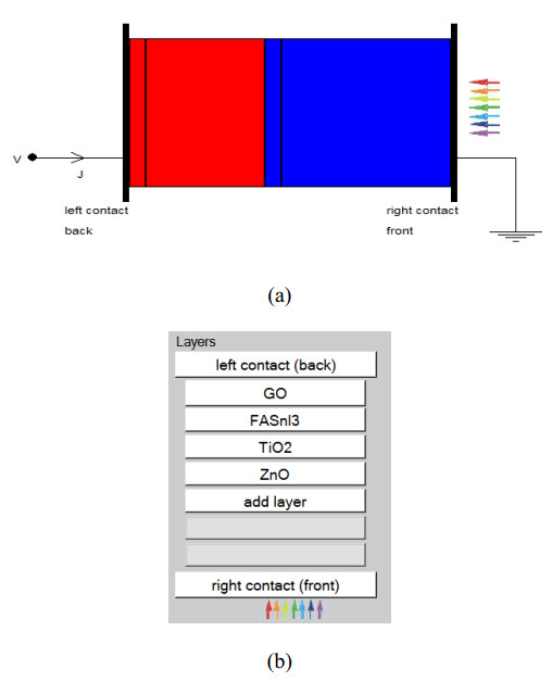
This paper focuses on the numerical study of hybrid organic-inorganic perovskite solar cells. It investigates the incorporation of a graphene oxide (GO) thin layer to enhance solar cell efficiency. The study demonstrates that the GO layer improves interaction with the absorber layer and enhances hole transportation, resulting in reduced recombination and diffusion losses at the absorber and hole transport layer (HTL) interface. The increased energy level of the Lower Unoccupied Molecular Orbital (LUMO) in GO acts as an excellent electron-blocking layer, thereby improving the V_OC. The objective is to explore different structures of perovskite solar cells to enhance their performance. The simulated solar cell comprises a GO/FASnI₃/TiO₂/ZnO/ITO sandwich structure, with FASnI₃ and ZnO thicknesses adjusted to improve conversion efficiency. The impact of thickness on device performance, specifically the absorber and electron transport layers, is investigated. The fill factor (FF) changes as the absorber and electron transport layers (ETL) increase. The FF is an important parameter that determines PSC performance since it measures how effectively power is transferred from the cell to an external circuit. The optimized solar cell achieves a short-circuit current density (J_SC) of 27.27 mA/cm², an open-circuit voltage (V_OC) of 2.76 V, a fill factor (FF) of 27.05% and the highest power conversion efficiency (PCE) of 20.39% with 400 nm of FASnI₃ and 300 nm of ZnO. These findings suggest promising directions for the development of more effective GO-based perovskite solar cells.
- solar cell,
- graphene oxide,
- perovskite,
- fill factor,
- power conversion efficiency,
- SCAPS
Citation: Norsakinah Johrin, Fuei Pien Chee, Syafiqa Nasir, Pak Yan Moh. Numerical study and optimization of GO/ZnO based perovskite solar cell using SCAPS[J]. AIMS Energy, 2023, 11(4): 683-693. doi: 10.3934/energy.2023034

Related Papers:

Abstract

This paper focuses on the numerical study of hybrid organic-inorganic perovskite solar cells. It investigates the incorporation of a graphene oxide (GO) thin layer to enhance solar cell efficiency. The study demonstrates that the GO layer improves interaction with the absorber layer and enhances hole transportation, resulting in reduced recombination and diffusion losses at the absorber and hole transport layer (HTL) interface. The increased energy level of the Lower Unoccupied Molecular Orbital (LUMO) in GO acts as an excellent electron-blocking layer, thereby improving the V_OC. The objective is to explore different structures of perovskite solar cells to enhance their performance. The simulated solar cell comprises a GO/FASnI₃/TiO₂/ZnO/ITO sandwich structure, with FASnI₃ and ZnO thicknesses adjusted to improve conversion efficiency. The impact of thickness on device performance, specifically the absorber and electron transport layers, is investigated. The fill factor (FF) changes as the absorber and electron transport layers (ETL) increase. The FF is an important parameter that determines PSC performance since it measures how effectively power is transferred from the cell to an external circuit. The optimized solar cell achieves a short-circuit current density (J_SC) of 27.27 mA/cm², an open-circuit voltage (V_OC) of 2.76 V, a fill factor (FF) of 27.05% and the highest power conversion efficiency (PCE) of 20.39% with 400 nm of FASnI₃ and 300 nm of ZnO. These findings suggest promising directions for the development of more effective GO-based perovskite solar cells.

References

[1]	Roy P, Kumar SN, Tiwari S, et al. (2020) A review on perovskite solar cells: Evolution of architecture, fabrication techniques, commercialization issues and status. Sol Energy 198: 665–688. https://doi.org/10.1016/j.solener.2020.01.080 doi: 10.1016/j.solener.2020.01.080
[2]	Izadi F, Ghobadi A, Gharaati A, et al. (2021) Effect of interface defects on high efficient perovskite solar cells. Optik 227: 166061. https://doi.org/10.1016/j.ijleo.2020.166061 doi: 10.1016/j.ijleo.2020.166061
[3]	Nowsherwan GA, Samad A, Iqbal MA, et al. (2022) Performance analysis and optimization of a PBDB-T: ITIC based organic solar cell using graphene oxide as the hole transport layer. Nanomater 12. https://doi.org/10.3390/nano12101767 doi: 10.3390/nano12101767
[4]	Tyagi S, Singh PK, Tiwari AK (2022) Photovoltaic parameter extraction and optimisation of ZnO/GO based hybrid solar trigeneration system using SCAPS 1D. Energy Sustainable Dev 70: 205–224. https://doi.org/10.1016/j.esd.2022.08.001 doi: 10.1016/j.esd.2022.08.001
[5]	Touafek N, Mahamdi R, Dridi C, et al. (2021) Boosting the performance of planar inverted perovskite solar cells employing graphene oxide as HTL. Dig J Nanomater Bios 16: 705–712. Available from: https://chalcogen.ro/705_TouafekN.pdf.
[6]	Nguang SY, Liew ASY, Chin WC, et al. (2022) Effect of graphene oxide on the energy level alignment and photocatalytic performance of Engelhard Titanosilicate-10. Mater Chem Phys 275: 125198. https://doi.org/10.1016/j.matchemphys.2021.125198 doi: 10.1016/j.matchemphys.2021.125198
[7]	Zyoud SH, Zyoud AH, Ahmed NM, et al. (2021) Numerical modeling of high conversion efficiency FTO/ZnO/CdS/CZTS/MO thin filmbased solar cells: Using Scaps-1D software. Crystals 11: 1468. https://doi.org/10.3390/cryst11121468 doi: 10.3390/cryst11121468
[8]	Wibowo A, Marsudi MA, Amal MI (2020) ZnO nanostructured materials for emerging solar cell applications. RSC Adv 10: 42838–42859. https://doi.org/10.1039/d0ra07689a doi: 10.1039/D0RA07689A
[9]	Zhang P, Wu J, Zhang T, et al. (2018) Perovskite solar cells with ZnO electron-transporting materials. Adv Mater 30: 1703737. https://doi.org/10.1002/adma.201703737 doi: 10.1002/adma.201703737
[10]	Bouich A, Marí-Guaita J, Soucase BM, et al. (2022) Manufacture of high-efficiency and stable lead-free solar cells through antisolvent quenching engineering. Nanomater 12: 2901. https://doi.org/10.3390/nano12172901 doi: 10.3390/nano12172901
[11]	Shafi MA, Khan L, Ullah S, et al. (2022) Novel compositional engineering for ~26% efficient CZTS-perovskite tandem solar cell. Optik 253: 168568. https://doi.org/10.1016/j.ijleo.2022.168568 doi: 10.1016/j.ijleo.2022.168568
[12]	Li S, Liu P, Pan L, et al. (2019) The investigation of inverted p-i-n planar perovskite solar cells based on FASnI₃ films. Sol Energy Mater Sol Cells 199: 75–82. https://doi.org/10.1016/j.solmat.2019.04.023 doi: 10.1016/j.solmat.2019.04.023
[13]	Yasin S, Moustafa M, Al Zoubi T, et al. (2021) High efficiency performance of eco-friendly C₂N/FASnI₃ double-absorber solar cell probed by numerical analysis. Opt Mater 122. https://doi.org/10.1016/j.optmat.2021.111743 doi: 10.1016/j.optmat.2021.111743
[14]	Kumar M, Raj A, Kumar A, et al. (2020) An optimized lead-free formamidinium Sn-based perovskite solar cell design for high power conversion efficiency by SCAPS simulation. Opt Mater 108: 110213. https://doi.org/10.1016/j.optmat.2020.110213 doi: 10.1016/j.optmat.2020.110213
[15]	Burgelman M, Decock K, Khelifi S, et al. (2013) Advanced electrical simulation of thin film solar cells. Thin Solid Films 535: 296–301. https://doi.org/10.1016/j.tsf.2012.10.032 doi: 10.1016/j.tsf.2012.10.032
[16]	Shi T, Zhang HS, Meng W, et al. (2017) Effects of organic cations on the defect physics of tin halide perovskites. J Mater Chem 5: 15124–15129. https://doi.org/10.1039/C7TA02662E doi: 10.1039/C7TA02662E
[17]	Ahmed MI, Hussain Z, Mujahid M, et al. (2016) Low resistivity ZnO-GO electron transport layer based CH₃NH₃PbI₃ solar cells. AIP Adv 6: 065303. https://doi.org/10.1063/1.4953397 doi: 10.1063/1.4953397
[18]	Kim MK, Jeon T, Park HI, et al. (2016) Effective control of crystal grain size in CH₃NH₃PbI₃ perovskite solar cells with a pseudohalide Pb(SCN)₂ additive. CrystEngComm 18: 6090–6095. https://doi.org/10.1039/c6ce00842a doi: 10.1039/C6CE00842A
[19]	Tao S, Schmidt I, Brocks G, et al. (2019) Absolute energy level positions in tin- and lead-based halide perovskites. Nat Commun 10: 2560. https://doi.org/10.1038/s41467-019-10468-7 doi: 10.1038/s41467-019-10468-7
[20]	Li S, Yang F, Chen M, et al. (2022) Additive engineering for improving the stability of tin-based perovskite (FASnI₃) solar cells. Sol Energy 243: 134–141. https://doi.org/10.1016/j.solener.2022.07.009 doi: 10.1016/j.solener.2022.07.009
[21]	Burgelman M, Decock K, Niemegeers A, et al. (2016) SCAPS manual. University of Ghent: Ghent, Belgium. Available from: https://scaps.elis.ugent.be/SCAPS%20manual%20most%20recent.pdf.
[22]	Alipour H, Ghadimi A (2021) Optimization of lead-free perovskite solar cells in normal-structure with WO₃ and water-free PEDOT: PSS composite for hole transport layer by SCAPS-1D simulation. Opt Mater 120. https://doi.org/10.1016/j.optmat.2021.111432 doi: 10.1016/j.optmat.2021.111432
[23]	Deepthi JK, Sebastian V (2021) Comprehensive device modelling and performance analysis of MASnI₃ based perovskite solar cells with diverse ETM, HTM and back metal contacts. Sol Energy 217: 40–48. https://doi.org/10.1016/j.solener.2021.01.058 doi: 10.1016/j.solener.2021.01.058
[24]	Bello IT, Idisi DO, Suleman KO, et al. (2022) Thickness variation effects on the efficiency of simulated hybrid Cu₂ZnSnS₄-based solar cells using Scaps-1D. Biointerface Res Appl Chem 12: 7478–7487. https://doi.org/10.33263/BRIAC126.74787487 doi: 10.33263/BRIAC126.74787487
[25]	Tara A, Bharti V, Sharma S, et al. (2021) Device simulation of FASnI₃ based perovskite solar cell with Zn(O_0.3, S_0.7) as electron transport layer using SCAPS-1D. Opt Mater 119: 111362. https://doi.org/10.1016/j.optmat.2021.111362 doi: 10.1016/j.optmat.2021.111362
[26]	Saeed F, Gelani HE (2022) Unravelling the effect of defect density, grain boundary and gradient doping in an efficient lead-free formamidinium perovskite solar cell. Opt Mater 124: 111952. https://doi.org/10.1016/j.optmat.2021.111952 doi: 10.1016/j.optmat.2021.111952
[27]	Ait-Wahmane Y, Mouhib H, Ydir B, et al. (2021) Comparison study between ZnO and TiO₂ in CuO based solar cell using SCAPS-1D. Mater Today: Proc 52: 166–171. https://doi.org/10.1016/j.matpr.2021.11.535 doi: 10.1016/j.matpr.2021.11.535
[28]	Sawicka-Chudy P, Sibiński M, Wisz G, et al. (2018) Numerical analysis and optimization of Cu₂O/TiO₂, CuO/TiO₂, heterojunction solar cells using SCAPS. J Phys Conf Ser https://doi.org/10.1088/1742-6596/1033/1/012002 doi: 10.1088/1742-6596/1033/1/012002
[29]	Mouchou RT, Jen TC, Laseinde OT, et al. (2021) Numerical simulation and optimization of p-NiO/n-TiO₂ solar cell system using SCAPS. Mater Today: Proc 38: 835–841. https://doi.org/10.1016/j.matpr.2020.04.880 doi: 10.1016/j.matpr.2020.04.880
[30]	Enebe G, Lukong V, Mouchou R, et al. (2022) Optimizing nanostructured TiO₂/Cu₂O pn heterojunction solar cells using SCAPS for fourth industrial revolution. Mater Today: Proc 62: S145–S150. https://doi.org/10.1016/j.matpr.2022.03.485 doi: 10.1016/j.matpr.2022.03.485
[31]	Ghosh BK, Nasir S, Chee FP, et al. (2022) Numerical study of nSi and nSiGe solar cells: Emerging microstructure nSiGe cell achieved the highest 8.55% efficiency. Opt Mater 129: 112539. https://doi.org/10.1016/j.optmat.2022.112539 doi: 10.1016/j.optmat.2022.112539
[32]	Guo X, Zhou N, Lou SJ, et al. (2013) Polymer solar cells with enhanced fill factors. Nat Photonics 7: 825–833. https://doi.org/10.1038/nphoton.2013.207 doi: 10.1038/nphoton.2013.207
[33]	Proctor CM, Kim C, Neher D, et al. (2013) Nongeminate recombination and charge transport limitations in diketopyrrolopyrrole-based solution-processed small molecule solar cells. Adv Funct Mater 23: 3584–3594. https://doi.org/10.1002/adfm.201202643 doi: 10.1002/adfm.201202643
[34]	Ryu S, Noh JH, Jeon NJ (2014) Voltage output of efficient perovskite solar cells with high open-circuit voltage and fill factor. Energy Environ Sci 7: 2614–2618. https://doi.org/10.1039/c4ee00762j doi: 10.1039/C4EE00762J
[35]	Rasmidi R, Mivolil DS, Chee FP, et al. (2022) Structural and optical properties of TIPS pentacene thin film exposed to gamma radiation. Mater Res 25. https://doi.org/10.1590/1980-5373-MR-2022-0227 doi: 10.1590/1980-5373-MR-2022-0227

Reader Comments

Your name:*

Email:*
© 2023 the Author(s), licensee AIMS Press. This is an open access article distributed under the terms of the Creative Commons Attribution License (http://creativecommons.org/licenses/by/4.0)