Effect of different washing conditions on the removal efficiency of selected compounds in biopolymers

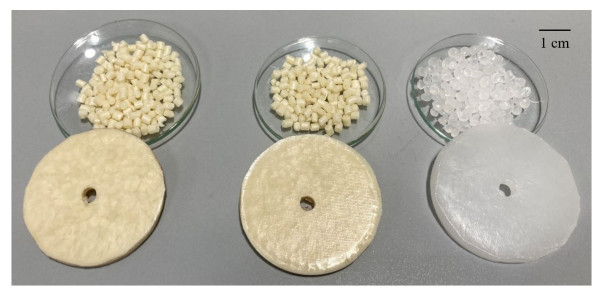
1.   Introduction

In the last few decades, fractional differential equations have become an active research topic due to their applications in many fields, such as computer science, biology, mechanics and nonlinear fractional-order Lorenz system^[1]. To date, many researchers have conducted in-depth research on several fractional order derivatives and integrals, such as Caputo, Riemann-Liouville, Riesz and so on. In ^[2], they develop an extension of a quadrature method for solving a class of $\psi$-fractional differential equations by converting them to an equivalent linear Volterra integral equation as follows:

The Caputo-Hadamard fractional integrals are the special forms for $\psi(t) = log(t)$ in (1.1). However, the Caputo-Hadamard fractional integrals are also very important for simulating different physical problems ^[3,4]. Recently, Caputo-Hadamard fractional differential integral equations have made a breakthrough in ^[5]. Therefore, in practice, the Caputo-Hadamard fractional integral equation is also worth further research. The purpose of this project was to construct an in-depth theory and application of the high-precision algorithm for Caputo-Hadamard fractional integral system on a uniform grid. To this end, we will study the following 2D nonlinear Caputo-Hadamard integral equation:

where $K (s, t, \tau, \omega, f(\tau, \omega))$, $g(s, t)$ are known functions and $f(s, t)$ is an unknown function in $\Theta = [a, b]\times [c, d]$, $\Omega = \Theta\times \Theta\times R$. We assume that the solution of (1.2) is smooth and $K(s, t, \tau, \omega, f(\tau, \omega)$ satisfies the Lipschitz condition about the fifth variable.

In ^[6], a solution of the Caputo-Hadamard fractional differential equation based on a hierarchical grid is presented. In ^[7], the solution's existence and uniqueness of fractional Caputo-Hadamard type equations are given. In an existing reference ^[8], we consider the logarithmic decay and regularity of solutions of Caputo-Hadamard fractional diffusion equations. In ^[9], a new stable and high order uniform accuracy solution method is given for 2D nonlinear integral equations. In ^[10], the fractional stochastic differential equations solution's existence and uniqueness was proved by the fixed point method in the Caputo-Hadamard sense. In ^[11], they present three types of variable fractional orders in the Caputo-Hadamard sense. In ^[12], numerical methods for the initial singularity fractional equations were investigated by using the modified Laplace transform and FFT in the Caputo-Hadamard sense. In ^[13], they used the incomplete Gamma function to construct the time discretization scheme for Caputo-Hadamard fractional differential equations. In ^[14], a local discontinuous Galerkin algorithm based on the Gronwall inequality is proposed for fractional differential equations in the sense of Caputo-Hadamard. In ^[15], a kind of graded grid algorithm in the sense of Caputo-Hadamard is studied. In ^[16], they established a method for solving Caputo-Hadamard integrals and a class of fractional derivatives by using the logarithmic transformation of Jacobian polynomials. The calculation methods for three fractional differentials in the sense of Caputo-Hadamard have been given in ^[17]. In ^[18], they use uncertain fractional derivatives to discuss the price of European options. The research of Caputo-Hadamard equation can be found in ^[19], the applicant uses the spectrum method to give an algorithm for sets of Caputo-Hadamard fractional PDE. In ^[20], a numerical method for time-space fractional discrete systems in the sense of Caputo-Hadamard is given. For more information, please refer to ^[21,22,23].

In this paper, we will use a uniform mesh to solve 2D nonlinear fractional Hadamard integral equations based on the idea of ^[9], achieving uniform accuracy by using piecewise biquadratic logarithmic interpolations. For $0 < \gamma, \lambda < 1$, we obtain an optimal convergence order of $O({\Delta_{s}^{4-\gamma }}+{\Delta_{t}^{4-\lambda }})$ for a sufficiently smooth solution and a generalized nonlinear kernel function by using the Gronwall inequality based on the convergence analysis of a new technique.

The framework of this article is as follows. In Section 2, we give a high precision numerical method. The truncation error of the high order numerical method is mainly discussed in Section 3. In Section 4, the convergence of the high order numerical scheme is analyzed. In Section 5, two numerical experiments are presented to support our theory and demonstrate the efficiency of higher-order numerical methods. The final section summarizes the main contribution of the work and the future research work.

2.   Higher-order numerical scheme using two-dimensional nonlinear fractional Hadamard integral equations

Now, we can obtain an approximate evaluation of the Caputo Hadamard integral equations in two dimensions. In order to construct a numerical scheme for (1.2), we partition the domain $\Theta$ into $2Y\times 2X$ subdomains of equal size $\Delta_{s} = \frac{b-a}{2Y}$ and $\Delta_{t} = \frac{d-c}{2X}$, where $Y$ and $X$ are positive integers. Assuming $s_n = a+n \Delta_s$ and $t_m = c+m \Delta_t$, $n = 0, 1, 2, \cdots, 2Y,$ $m = 0, 1, 2, \cdots, 2X$ with $a, c \geq 1$, where $a = s_0 < s_1 < \cdots < s_{2Y} = b$ and $c = t_0 < t_1 < \cdots < t_{2X} = d$ are respective partitions of $\left[a, b\right]$ and $\left[c, d\right]$. And we use ${{f}_{n}^{m}}$ to represent a numerical scheme for (1.2) at a point $({{{s}_{n}}, {{t}_{m}}})$, and we let ${{K }_{n}^{m}}{(\tau, \omega, f(\tau, \omega))} = K ({{s}_{n}}, {{t}_{m}}, \tau, \omega, f(\tau, \omega))$ and $g_{n}^{m} = g(s_{n}, t_{m})$.

In this work, we present a high-order method for solving nonlinear fractional Hadamard integral equations. The basis functions of our approach are determined by the quadratic logarithmic interpolations of polynomials at points ${{s}_{n}}, {{s}_{n+1}}, {{s}_{n+2}}$ and ${{t}_{m}}, {{t}_{m+1}}, {{t}_{m+2}}$, and they are assumed to be ${{\varphi }_{k}^{n}}(\tau), k = 0, 1, 2; n\in \mathbb{N}$ and ${{\phi }_{k}^{m}}(\omega), k = 0, 1, 2; m\in \mathbb{N}$, respectively, and they are defined as follows:

In what follows, we construct the numerical scheme approximation to $f(s, t)$ at a point $(s_{1}, t_{1})$:

with

Similarly, we compute $f(s_{2}, t_{1}), f(s_{1}, t_{2})$ and $f(s_{2}, t_{2})$ to obtain the following approximate values:

where

We need to compute $f_{1}^{1}$ through the use of (2.1) by using the values of $K$ at $s_1, s_2$ and $t_1, t_2$. Particularly the dependence of $f_{1}^{1}$ on $K_{2}^{1}, K_{1}^{2}$ and $K_{2}^{2}$ means that (2.1) and (2.3)–(2.5) must be couple solved with the scheme.

Next, we estimate $f(s_{2y+l}, t_r), y = 1, \cdots, Y-1$ and $f(s_l, t_{2x+r}), l, r = 1, 2, x = 1, \cdots, X-1$. Assuming that $f_{n}^{r}, n = 0, 1, \cdots, 2y$ and $f_{l}^{m}, m = 0, 1, \cdots, 2x$ are known, we have $f(s_{2y+1}, t_1)$:

where $\hat T_1^{q, 0}$ is given by (2.2) and

For $f(s_{2y+2}, t_1)$ and $f(s_{2y+l}, t_2), l = 1, 2$, we use the following approximate estimates:

where $\hat T_1^{q, 0}, \hat T_2^{q, 0}, T_{2y+1}^{k, 0}, T_{2y+1}^{k, n}$ are defined by (2.2), (2.6), (2.8) and (2.9), respectively, and $T_{2y+2}^{k, n}$ is defined as follows:

In the same way, we estimate $f(s_l, t_{2x+r})$ for $l, r = 1, 2$ as follows:

where $T_2^{k, 0}$ and $T_1^{k, 0}$ are given by (2.6) and (2.2), respectively, and

Similarly, when ${{f}_{n}^{m}}, {{f}_{n}^{2x+1}}, {{f}_{n}^{2x+2}},$ ${{f}_{2y+1}^{m}}$ and ${{f}_{2y+2}^{m}}, n = 0, 1, \cdots, 2y;m = 0, 1, \cdots, 2x;y = 1, \cdots,$ $Y-1;x = 1, \cdots, X-1$ are already known, we will construct the high order scheme for $f({{s}_{2{y+p}}}, {{t}_{2x+q}}), p, q = 1, 2$ as follows.

For $f(s_{2y+1}, t_{2x+1})$, we have

For ${{F}_{1}}$, by using biquadratic interpolation one can obtain

where $T_{2y+1}^{k, 0}$ and $\hat{T}_{2x+1}^{q, 0}$ are defined by (2.8) and (2.18), respectively.

For ${{F}_{2}}$, through direct calculation, it can be concluded that

where $T _{2y+1}^{k, 0}$ and $\hat{T }_{2x+1}^{q, m}$ are given by (2.8) and (2.19), respectively.

For $F_3$, one can obtain that

where $T_{2y+1}^{k, n}$ and $\hat{T }_{2x+1}^{q, 0}$ are given by (2.9) and (2.18), respectively.

Similarly, for $F_4$, we have

where $T_{2y+1}^{k, n}$ and $\hat{T }_{2x+1}^{q, m}$ are given by (2.9) and (2.19), respectively.

Bringing (2.22)–(2.25) into (2.21), one can obtain

Furthermore, we will construct a high order numerical scheme for $f(s_{2y+2}, t_{2x+1})$. By dividing the integral domain into subdomains and using the piecewise biquadratic interpolation method, we calculate $f(s_{2y+2}, t_{2x+1})$ as follows

where $T_{2y+2}^{k, n}$ is defined by (2.13) and $\hat{T }_{2x+1}^{q, 0}$ and $\hat{T}_{2x+1}^{q, m}$ are given by (2.18) and (2.19), respectively.

Therefore, we can obtain an approximation of $f({{s}_{2y+1}}, {{t}_{2x+2}})$ and $f({{s}_{2y+2}}, {{t}_{2x+2}})$ as follows

where $T _{2y + 1}^{k, 0}$, $T_{2y+1}^{k, n}$, $T_{2y+2}^{k, n}$ and $\hat{T}_{2x+2}^{q, m}$ are given by (2.8), (2.9), (2.13) and (2.20), respectively.

In summary, we combine (2.1), (2.3)–(2.5), (2.7), (2.10)–(2.12), (2.14)-(2.17) and (2.26)–(2.29) to obtain the high-order numerical scheme of (1.2) as follows

3.   Estimation of the truncation errors

We will introduce several lemmas that will be used in convergence analysis. In the this paper, we assume that $C$ is a constant; the value of $C$ may vary at different positions and it is independent of the discrete step size.

Lemma 1. (Discrete Gronwall Inequality ^[24]) Assume that $0 < \gamma < 1$ and $b > a > 0$, and

Let $\sum\limits_{n = p}^y a_{n, y}\left|e_n\right| = 0$ for $p > y \geq 1$. If

then

where $A$ and $C$ are positive constants.

Lemma 2. ^[25] For $g > f > 0$, the following holds

where $\gamma > 0, \lambda > 0$.

Based on the idea of ^[25], we can prove the following Lemma 3–Lemma 5.

Lemma 3. It holds that

where $r > n$ and $b$ is a positive constant.

Lemma 4. Let $n > m$ and $p > q$; then,

Lemma 5. Assuming that $p$ and $q$ are positive integers and $p, q = 0, 1, 2, \cdots, 2y+1$, when $p > q$ is satisfied, the following conclusion holds:

In order to estimate the truncation error for (2.30), we introduce the definition of truncation error at a point $(s_n, t_m)$:

where ${\bar f_{n}^{m}}$ is used as an approximation of $f({{s_{n}}, {t_{m}}})$ in order to obtain a precise solution when substituted into (2.30). Specifically, ${\bar f_{2y + 1}^{2x + 1}}$ is defined by

Lemma 6. Let ${r_{n}^{m}}$ represent the definition of truncation error in (3.2). If $K (\cdot, \cdot, \cdot, \cdot, f(\cdot, \cdot)) \in {C^4}([a, b] \times [c, d])$, then we have

where $C$ is only related to $\gamma, \lambda, {{G}_{1}}, {{G}_{2}}$, and the respective definitions of $G_1, G_2$ are as follows:

Proof. Let us first estimate the truncation error ${r_{2y + 1}^{2x + 1}}$. From (3.2), it can be seen that the truncation error has already been defined at the point $(s_{2y+1}, t_{2x+1})$. By combining (2.26), (3.2) and (3.3), it can be obtained that

We can obtain the following from Taylor's theorem for all $(\tau, \omega)\in [a, {{s}_{1}}]\times [c, {{t}_{1}}]$:

where $({{\xi }_{1}}(\tau), {{\eta }_{1}}(\omega))\in [a, {{s}_{1}}]\times [c, {{t}_{1}}]$. For all $(\tau, \omega)\in [a, {{s}_{1}}]\times [{{t}_{2m-1}}, {{t}_{2m+1}}]$ with $({{\xi }_{2}}(\tau), {{\eta }_{m}}(\omega))\in [a, {{s}_{1}}]\times [{{t}_{2m-1}}, {{t}_{2m+1}}]$, then

and for all $(\tau, \omega)\in [{{s}_{2n-1}}, {{s}_{2n+1}}]\times [c, {{t}_{1}}]$, there exists $({{\xi }_{n}}(\tau), {{\eta }_{2}}(\omega))\in [{{s}_{2n-1}}, {{s}_{2n+1}}]\times [c, {{t}_{1}}]$, such that

In the same way, for all $(\tau, \omega)\in [{{s}_{2n-1}}, {{s}_{2n+1}}]\times [{{t}_{2m-1}}, {{t}_{2m+1}}]$, there exists $({{\xi }_{n1}}(\tau), {{\eta }_{m2}}(\omega))\in [{{s}_{2n-1}}, {{s}_{2n+1}}]\times [{{t}_{2m-1}}, {{t}_{2m+1}}]$, such that

So, we can obtain the value of $r_{2y+1}^{2x+1, (1)}$ as follows

For the convenience of estimating of each item on the right side of (3.7), according to Lemma 3 and Lemma 5, let us first estimate the following:

Similarly, we have

Then we have

where $a < \delta < s_1$ and $c < \rho < t_1$; $G_1$ is defined by (3.4).

By combining (3.10) and (3.11), it is easy to conclude that

Similarly, for $r_{2y+1}^{2x\text{+}1, (2)}$, we use the same technique to obtain

For $R_{2}^{(1)}$ of (3.13), based on (3.8) and Lemma 5 we can see that

For $R_{2}^{(2)}$, we decompose it into the following estimates

where ${{\tilde{\omega}}_{m}}{ = }{{t}_{2m}}$. Based on ${\varphi}_{k}^{n}(\tau), \tau\in(s_{n}, s_{n+2}), k = 0, 1, 2;n\in\mathbb{N}$, we derive $|{\varphi}_{k}^{n}(\tau)|\le1$ by using (3.8); so, we have the following inequality

For $D_{11}$, we can obtain that

where ${{\log \hat{ \omega}}_{m}}\le {{log \omega}_{m}}\le {{\log \bar{\omega}}_{m}}$, ${{\log t}_{2m-1}}\le {{\log \hat{\omega}}_{m}}\le {{\log t}_{2m}}\le{{\log \bar{\omega}}_{m}}\le {{\log t}_{2m+1}}$. Furthermore, $2x-1 \ge 3$; then, $x$ satisfies that $x \ge 2$, so we know that $t_{2x-1} \ge t_3 = c+3 \Delta_{t}$; then, $\frac{ \Delta_{t}}{t_{2x-1}} \le \frac{1}{3}$, $1-\frac{\Delta_t}{t_{2x-1}} \ge \frac{2}{3}$, and we have that $\frac{ 2 \Delta_{t}}{t_{2x-1}} \Big(1-\frac{ \Delta_t}{t_{2x-1}}\Big) \ge \frac{4}{3} \frac{\Delta_t}{t_{2x-1}}$.

For $D_{12}$, one can similarly obtain that

We substitute (3.17) and (3.18) into (3.16) to obtain $D_{1}$:

So, we get $D_{2}$:

where $G_2$ is defined by (3.5).

According to (3.19) and (3.20), (3.15) becomes

By combining (3.14) and (3.21) with (3.13) we can obtain the result of $r_{2y+1}^{2x+1, (2)}$ as follows:

Next, we estimate $r_{2y+1}^{2x{+}1, (3)}$ and obtain

For $R_{3}^{(1)}$, one can obtain that

where ${{\tilde{\tau}}_{n}} = {{s}_{2n}}$.

For $B_{1}$, we obtain

According to (3.17) and (3.18), we can use the same method to obtain the forms of $B_{11}$ and $B_{12}$ as follows

So, $B_{1}$ can be directly obtained

For ${B}_{2}$, similar to $D_2$, we can also directly obtain

According to (3.23) and (3.24), we have

Next, let us estimate $R_{3}^{(2)}$ as follows

So according to (3.25) and (3.26), we can obtain $r_{2y+1}^{2x+1, (3)}$ as follows

We estimate $r_{2y+1}^{2x+1, ({4})}$ and obtain the following form

We conducted detailed estimates for $R_{4}^{(1)}$ and $R_{4}^{(2)}$ respectively, and obtained $R_{4}^{(1)}$

where ${{\tilde{\tau}}_{n}} = {{s}_{2n}}$; using the same processing method as $B_{1}$, we can obtain ${N}_{1}$ as follows:

Therefore, for $N_{2}$, it can be obtained that

Finally, Let us estimate $R_{4}^{(2)}$ again

where ${{\tilde{\omega}}_{m}}{ = }{{t}_{2m}}$. $V_{1}$ and $V_{2}$ are denoted as the two terms at the right end of the above formula. Refer to $D_{1}$ and use the same method to obtain $V_{1}$:

So, $r_{2y+1}^{2x+1, (4)}$ is obtained as follows

We then substitute (3.12) and (3.22)–(3.28) into (3.6) and calculate the form of ${{r}_{2y+1}^{2x+1}}$ as follows

The constant $C$ only relies on ${{G}_{1}}, {{G}_{2}}, \gamma$ and $\lambda$.

Similar to ${{r}_{2y+1}^{2x+1}}$, we can prove that

Therefore, we conclude that the truncation error ${{r}_{n}^{m}}$ satisfies the following conditions:

The proof is thus completed. □

4.   Convergence analysis

In this section, to simplify the symbols for convergence analysis, we introduce the following coefficients to rewrite the numerical scheme; carefully observing (2.9), (2.13), (2.19) and (2.20), it is obvious that $T_{2y+1}^{k, n} = T_{2y+2}^{k, n}, k = 0, 1, 2, n = 1, 2, \cdots, y$ and $\hat{T}_{2x+1}^{q, m} = \hat{T}_{2x+2}^{q, m}, q = 0, 1, 2, m = 1, 2, \cdots, x$. Therefore, we can use the following equivalent form to recalculate the numerical scheme (2.30):

where $y = 1, \ 2, \ \cdots, \ Y-1$; $x = 1, \ 2, \ \cdots, \ X-1$, and

Next, we propose Lemma 7.

Lemma 7. The coefficients of $\bar{Q}_{n}^{y}, n = 0, 1, \cdots, 2y+1$, and $\bar{W}_{m}^{x}, m = 0, 1, \cdots, 2x+1$, are shown in (4.2), and they satisfy

Proof. This proves the estimate of (4.3) for $n = 0$; using Lemma 3, we have

where $a < \xi_1 < s_{2y+1} < b, a < s_1 < \xi_2 < s_{2y+1} < b$ and $C$ is independent on $\Delta_t$.

For $n = 1$, using Lemma 3 and Lemma 7, we have

Next, for $n = 2$, we obtain

On one side, using Lemma 3, we have

On the other side,

So, we have

Next, we will estimate $\left|\bar{Q}_{n}^{y}\right|, n = 3, \cdots, 2 y$. For $n = 2 r+1, r = 1, 2, \cdots, y-1$, we obtain

For $n = 2 r, r = 2, \cdots, y$, we have

Next, let us prove (4.4). According to Lemma 2, we proceed as follows:

So we can get

where $\left(\log \frac{s_{2 y+1}}{s_{2 y-1}}\right)^{1-\gamma} = \left(\log \Big(1+\frac{{2\Delta_s}}{s_{2 y-1}}\Big)\right)^{1-\gamma} \leq\left(\frac{{2\Delta_s}}{s_{2 y-1}}\right)^{1-\gamma}\leq\left(\frac{{2\Delta_s}}{{a}}\right)^{1-\gamma}$. Taking all of the results together, we can obtain the estimates (4.3) and (4.4). □

Since the proof process for $\bar{Q}_{n}^{y}$ is the same as that for $\bar{W}_{m}^{y}$, we will omit it without further proof.

Lemma 8. The coefficients of ${Q}_{n}^{y}, n = 0, 1, \cdots, 2y+2$, and ${W}_{m}^{x}, m = 0, 1, \cdots, 2x+2$, satisfy

Proof. The proof process for Lemma 8 can be achieved by referring to the method used in Lemma 7. □

Next, we analyze the convergence by using the scheme (4.1), as in the following Theorem 1.

Theorem 1. Let $u$ be the solution of (1.2) and ${f}_{n}^{m}$ $(n = 0, 1, \cdots, 2Y$, $m = 0, 1, \cdots, 2X)$ be the numerical solution of (1.2) by using scheme (4.1). Assume that $K (\cdot, \cdot, \cdot, \cdot, f(\cdot, \cdot))\in {{C}^{4}}([a, b]\times [c, d]\times R)$ satisfies (1.3) and $\Delta_s$, $\Delta_t$ satisfy

Then the error is that

where $C$ is constant and only dependent on $L, K, b, d, \gamma$ and $\lambda$.

Proof. Assume that ${{e}_{i}^{m}} = f({{s}_{n}}, {{t}_{m}})-{{f}_{n}^{m}}, n = 0, 1, \cdots, 2Y; m = 0, 1, \cdots, 2X$. ${{e}_{n}^{0}} = {{e}_{0}^{m}} = 0$ can be readily observed. First, ${{e}_{n}^{m}}, n, m = 1, 2$, it can be known that

The calculation can prove that ${{\hat{Q}}_{n}}, {{\tilde{Q}}_{n}}, n = 0, 1, 2$, and (1.3) are satisfied by $K$, and that ${{\hat{W}}_{m}}, {{\tilde{W}}_{m}}, m = 0, 1, 2,$ are bounded. So, we come to the following conclusion:

We combine these four inequalities and obtain

Second, $e_{n}^{m}, n\ge 3;m = 1, 2,$ satisfies

It can be seen that the above four equations are coupled, so they need to be solved simultaneously. For convenience, we assume that $\left||\hat e_n\right\| = \max\{|e_{n}^{1}|, |e_{n}^{2}|, n = 0, 1, \cdots, 2Y\}$ and $\left||\hat r_n\right\| = \max\{|r_{y}^{1}|, |r_{y}^{2}|$, $y = 0, 1, \cdots, 2Y\}$. According to (1.3), (4.3) in Lemma 7, (4.10) and (4.11) in Lemma 8, (4.16) and (4.18) becomes

By Lemma 4, and through careful calculation, we have

Therefore, (4.20) becomes

Using the above same method, the estimates (4.17) and (4.19) are as shown below

For $\left\|\hat e_{2y+1}\right\|$, it is easy to verify that $\|\hat e_0\| = 0$; then we have

For enough small $\Delta_s$, we obtain

Applying Lemma 1 to (4.21) leads to

Using the same argument for $\left\|\hat e_{2y+2}\right\|$, we can directly conclude that there are some $C$ that

Now, based on the above results and Lemma 6, we can reach the following conclusion.

Next, satisfy ${{e}_{n}^{m}}, n, m\geq3$ to obtain

where ${{\bar{Q}}_{n}^{y}}, {{Q}_{n}^{y}}, {{\bar{W}}_{m}^{x}}$ and ${{W}_{m}^{x}}$ satisfy Lemma 6 and Lemma 7.

For ${e}_{2y+1}^{2x+1}$, we can obtain that

We rearrange it into the following form

If we let $\left\|{{{e}}_{n}}\right\| = \underset{0\le m\le 2X}{\mathop{\max }}\, |{{e}_{n}^{m}}|$ and $\left\|{{{r}}_{n}}\right\| = \underset{0\le m\le 2X}{\mathop{\max }}\, |{{r}_{n}^{m}}|$, we can conclude that

Then we have

According to (4.11) in Lemma 8, for enough small $\Delta_s$, we obtain,

According to (4.13) in Lemma 8, for enough small $\Delta_t$, let $\Delta_t < d$, so we have

Then, it follows from the Gronwall inequality introduced in Lemma 1 that

From Lemma 6, we can conclude that

Similarly, we can also obtain

We jointly establish (4.22), (4.23), (4.25) and (4.26); with this, we complete the proof of Theorem 1. □

5.   Numerical examples

Now, this section applies the numerical scheme to solve the 2D fractional Caputo-Hadamard integral equation. We present two calculation examples to demonstrate its effectiveness.

Example 5.1 Take into account the subsequent equation, which is linear 2D fractional Caputo-Hadamard integral equations:

where $a = 1$, $c = 1$, $b = 2$ and $d = 2$, and

where $f(s, t) = ({\log s})^{4}({\log t})^{4}$ is the exact solution.

We choose separately $\gamma = 0.3, \lambda = 0.6$ and $\gamma = 0.4, \lambda = 0.5$ to conduct experiments. $\Delta_{s} = \frac{ b- a}{2Y}$ is the size of the step taken in the direction of $s$, while $\Delta_{t} = \frac{ d- c}{2X}$ is the width of the step taken in the direction of $t$. For errors, we define them as follows

In this example, we test the convergence order for different values of $\gamma$ and $\lambda$ where the convergence order is determined as $\log_{2}(e_{2h}^f/e_{h}^f)$. The application of Theorem 1 allows us to determine the theoretical convergence order of the numerical scheme as $O({\Delta_{s}^{4-\gamma}}+{\Delta_{t}^{4-\lambda}})$. By considering $\Delta_{s}$ to be significantly smaller than $\Delta_{t}$, we can deduce that $O({\Delta_{s}^{4-\gamma }}+{\Delta_{t}^{4-\lambda}}) = O({\Delta_{t}^{4-\lambda}})$. Tables 1 presents the values of $\gamma = 0.3, \lambda = 0.6$, $\gamma = 0.4, \lambda = 0.5$ and $Y = 2X$ with the theoretical order $4-\lambda$. When $\gamma = 0.3$ and $\lambda = 0.6$, the theoretical convergence order is 3.4. Similarly, the theoretical convergence order is 3.5 for $\gamma = 0.4$ and $\lambda = 0.5$.

Similarly, we use the proposed numerical scheme in another way to verify the convergence order of the test. We take $X = [Y^{\frac{4-\gamma}{4-\lambda}}]$, where $[\cdot]$ represents rounding, and the theoretical order $O({\Delta_{s}^{4-\gamma }}+{\Delta_{t}^{4-\lambda }}) = O({\Delta_{t}^{4-\gamma }})$ of the numerical scheme. In Table 2, when $\gamma = 0.3$ and $\lambda = 0.6$, it is easy to see that the numerical results of the test are close to 3.7, and the test results indicate that when $\gamma = 0.4$ and $\lambda = 0.5$, the numerical values are approximately 3.6. By referring to Tables 1 and 2, it is easy to see that the high-order numerical scheme results in a convergence order of $O({\Delta_{s}^{4-\gamma }}+{\Delta_{t}^{4-\lambda }})$.

Next, let us draw an error distribution map with $Y = 2X, X = 128$. As shown in Figure 1, the error distribution of $\alpha = 0.3, \beta = 0.6$ is on the left, while the error distribution of $\alpha = 0.4, \beta = 0.5$ is on the right. In addition, we can easily see that the error can be as small as $10^{-7}$, indicating that the approximate value is very close to the exact value.

Example 5.2 Take into account the 2D nonlinear fractional Caputo-Hadamard integral equation as follows:

where $a = 1$, $c = 1$, $b = 2$ and $d = 2$, and

where $f(s, t) = ({\log s})^{3}({\log t})^{2}$ is the exact solution.

In Table 3, given $\gamma = 0.3, \lambda = 0.6$ and $\gamma = 0.4, \lambda = 0.5$, our experimental results closely match the expected values of 3.4 and 3.5, respectively. In Table 4, when $\gamma = 0.3$ and $\lambda = 0.6$, the experimental results closely mirror the theoretical value of 3.7, and when $\gamma = 0.4$ and $\lambda = 0.5$, the experimental results align closely with the projected value of 3.6. It is easy to see that the high-order numerical scheme results in a convergence order of $O({\Delta_{s}^{4-\gamma }}+{\Delta_{t}^{4-\lambda }})$.

Finally, let us draw an error distribution map with $Y = 2X, X = 128$. As shown in Figure 2, the error distribution of $\alpha = 0.3, \beta = 0.6$ is on the left, while the error distribution of $\alpha = 0.4, \beta = 0.5$ is on the right. In addition, we can easily see that the error can be as small as $10^{-10}$.

6.   Concluding remarks

Based on the idea of the modified block-by-block method of^[6], we have proposed a uniform accuracy high-order scheme (2.30) to approximate the 2D nonlinear Hadamard Volterra integral equation. A high-order numerical scheme was constructed by using the piecewise biquadratic interpolation. The uniform accuracy high-order scheme in the present article is an explicit and high efficiency scheme except for two boundary layers which are solved by implicit and coupled. Based on the test results of the above example, one can see that the convergence order is $O({\Delta_{s}^{4-\gamma }}+{\Delta_{t}^{4-\lambda }})$. We conducted a detailed error analysis of the high-order numerical scheme and confirmed the accuracy of the theoretical analysis through numerical examples and experiments. Through extensive analysis of this work, it can be seen that the numerical scheme (2.30) has the advantages of high accuracy, easy calculation and implementation, and it does not require coupled solutions. In future work, we intend to use a Fourier spectral method to solve such problems. Based on the ideas in ^[5,26], we found that high-order numerical non-uniform grids can be used to solve fractional order integral differential equation problems as follows

In addition, deep learning can also provide solutions for such problems, so research on this topic is very challenging.

Use of AI tools declaration

The authors declare that they have not used Artificial Intelligence (AI) tools in the creation of this article.

Acknowledgments

This work was supported by the National Natural Science Foundation of China (Grant Nos. 11961009, 12361083), the Natural Science Research Project of the Department of Education of Guizhou Province (Grant Nos. QJJ2023012, QJJ2023061, QJJ2023062) and the Natural Science Foundation of Fujian Province of China (Grant No. 2022J01338).

Conflict of interest

The authors declare that they have no competing interests.