Sudden variability in solar photovoltaic (PV) power output to electrical grid can not only cause grid instability but can also affect power and frequency quality. Therefore, to study the balance of electrical grid or micro-grid power generated by PV systems in an upstream direction, predicting models can help. The power output conversion is directly proportional to the solar irradiance. Unlike time horizons predictions, many technics of irradiance forecasting have been proposed, long, medium and short term forecasting. For the Island of Mauritius in the Indian Ocean, and regards to key policy decisions, the government has outlined its intention to promote the PV technologies through the local electricity supplier but oversee the technical requirements of PV power output predicts for 1 hour to 15-minutes ahead. So, this paper is illustrating results of the Johansen vector error correction model (VECM) cointegration approach, from the author original and previous studies, but for a very short term prediction of 15-minutes to PV power output in Mauritius. The novelty of this study, is the long run equilibrium relationship of the Johansen model, that was initially determined in previous research works and from dataset in Reunion Island, is then applied to the PV plant in the Island of Mauritius. The proposed prediction model is trained for an hourly and 15-minutes period from year 2019 to year 2022 for a random month and a random day. The experimental results show that the performance metric R2 values are more than 93% signifying that Johansen model is positively and strongly correlated to onsite measurements. This proposed model is a powerful predicting tool and more accuracy should be attained when associated to a machine learning method that can learn from datasets.
Citation: Harry Ramenah, Abdel Khoodaruth, Vishwamitra Oree, Zahiir Coya, Anshu Murdan, Miloud Bessafi, Damodar Doseeah. Johansen model for photovoltaic a very short term prediction to electrical power grids in the Island of Mauritius[J]. Clean Technologies and Recycling, 2023, 3(2): 107-118. doi: 10.3934/ctr.2023007
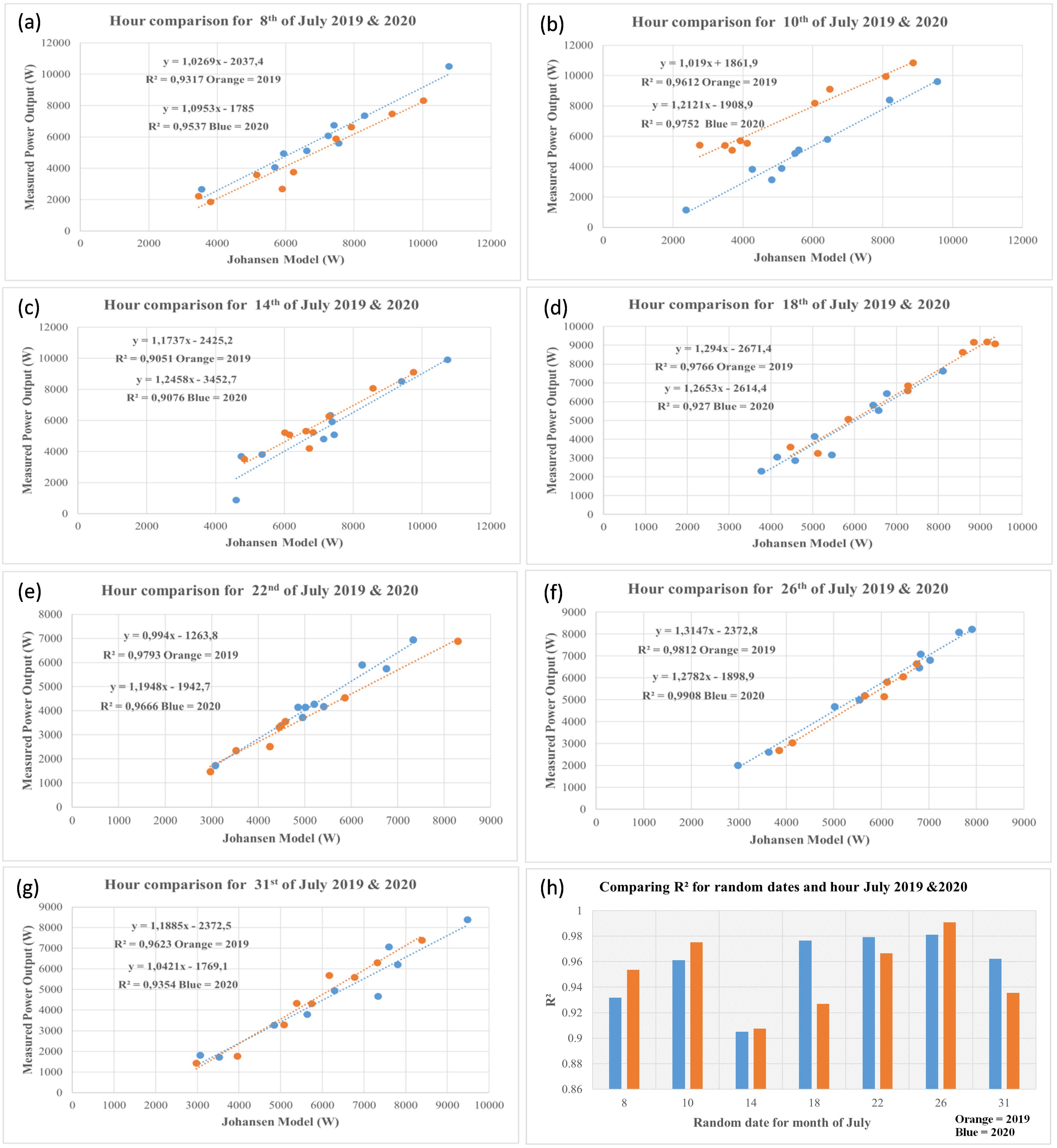
Sudden variability in solar photovoltaic (PV) power output to electrical grid can not only cause grid instability but can also affect power and frequency quality. Therefore, to study the balance of electrical grid or micro-grid power generated by PV systems in an upstream direction, predicting models can help. The power output conversion is directly proportional to the solar irradiance. Unlike time horizons predictions, many technics of irradiance forecasting have been proposed, long, medium and short term forecasting. For the Island of Mauritius in the Indian Ocean, and regards to key policy decisions, the government has outlined its intention to promote the PV technologies through the local electricity supplier but oversee the technical requirements of PV power output predicts for 1 hour to 15-minutes ahead. So, this paper is illustrating results of the Johansen vector error correction model (VECM) cointegration approach, from the author original and previous studies, but for a very short term prediction of 15-minutes to PV power output in Mauritius. The novelty of this study, is the long run equilibrium relationship of the Johansen model, that was initially determined in previous research works and from dataset in Reunion Island, is then applied to the PV plant in the Island of Mauritius. The proposed prediction model is trained for an hourly and 15-minutes period from year 2019 to year 2022 for a random month and a random day. The experimental results show that the performance metric R2 values are more than 93% signifying that Johansen model is positively and strongly correlated to onsite measurements. This proposed model is a powerful predicting tool and more accuracy should be attained when associated to a machine learning method that can learn from datasets.

| [1] |
Eom H, Son Y, Choi S (2020) Feature-selective ensemble learning-based long-term regional PV generation forecasting. IEEE Access 8: 54620–54635. https://doi.org/10.1109/ACCESS.2020.2981819 doi: 10.1109/ACCESS.2020.2981819

|
| [2] |
Lundquist K, Chow F, Lundquist J (2010) An immersed boundary method for the weather research and forecasting model. Mon Weather Rev 138: 796–817. https://doi.org/10.1175/2009MWR2990.1 doi: 10.1175/2009MWR2990.1
|
| [3] |
Chaturvedi DK (2016) Solar power forecasting: A review. Int J Comput Appl 145: 28–50. https://doi.org/10.5120/ijca2016910728 doi: 10.5120/ijca2016910728
|
| [4] |
Chow SKH, Lee EWM, Li DHW (2012) Short term prediction of photovoltaic energy generation by intelligent approach. Energ Buildings 55: 660–667. https://doi.org/10.1016/j.enbuild.2012.08.011 doi: 10.1016/j.enbuild.2012.08.011
|
| [5] |
Johansen S (1988) Statistical analysis of cointegration vectors. J Econ Dyn Control 12: 231–254. https://doi.org/10.1016/0165-1889(88)90041-3 doi: 10.1016/0165-1889(88)90041-3
|
| [6] |
Johansen S, Juselius K (1990) Maximum likelihood estimation and inferences on cointegration with applications to the demand for money. Oxford B Econ Stat 52: 169–210. https://doi.org/10.1111/j.1468-0084.1990.mp52002003.x doi: 10.1111/j.1468-0084.1990.mp52002003.x
|
| [7] |
Amri F (2017) The relationship amongst energy consumption (renewable and nonrenewable). Renewable Sustainable Energy Rev 76: 62–71. https://doi.org/10.1016/j.rser.2017.03.029 doi: 10.1016/j.rser.2017.03.029
|
| [8] |
Youssef YM, Belaïd F (2017) Environmental degradation, renewable and non-renewable electricity consumption, and economic growth: Assessing the evidence from Algeria. Energ Policy 102: 277–287. https://doi.org/10.1016/j.enpol.2016.12.012 doi: 10.1016/j.enpol.2016.12.012
|
| [9] | Kim H, Heo E (2012) Causality between main product and byproduct prices of metals used for thin-film PV cells. Proceedings of the 3rd IAEE Asian Conference, Kyoto, Japan, 1–9. |
| [10] |
Marques AC, Fuinhas JA, Menegaki AN (2014) Interactions between electricity generation sources and economic activity in Greece: A VECM approach. Appl Energ 132: 34–46. https://doi.org/10.1016/j.apenergy.2014.06.073 doi: 10.1016/j.apenergy.2014.06.073
|
| [11] |
Cano A, Arévalo P, Benavides D, et al. (2022) Comparative analysis of HESS (battery/supercapacitor) for power smoothing of PV/HKT, simulation and experimental analysis. J Power Sources 549: 232137. https://doi.org/10.1016/j.jpowsour.2022.232137 doi: 10.1016/j.jpowsour.2022.232137
|
| [12] |
Benavides D, Arévalo P, Tostado-Véliz M, et al. (2022) An experimental study of power smoothing methods to reduce renewable sources fluctuations using supercapacitors and lithium-ion batteries. Batteries 8: 228. https://doi.org/10.3390/batteries8110228 doi: 10.3390/batteries8110228
|
| [13] |
Ramenah H, Casin P, Ba M, et al. (2018) Accurate determination of parameters relationship for photovoltaic power output by Augmented Dickey Fuller test and Engle & Granger method. AIMS Energy 6: 19–48. https://doi.org/10.3934/energy.2018.1.19 doi: 10.3934/energy.2018.1.19
|
| [14] | Fanchette Y, Ramenah H, Casin P, et al. (2019) Predictive causality of Granger test for long run equilibrium to photovoltaic system. 2019 10th IEEE International Conference on Intelligent Data Acquisition and Advanced Computing Systems: Technology and Applications (IDAACS), Metz, France, IEEE, 942–946. https://doi.org/10.1109/IDAACS.2019.8924303 |
| [15] |
Fanchette Y, Ramenah H, Tanougast C, et al. (2020) Applying Johansen VECM cointegration approach to propose a forecast model of photovoltaic power output plant in Reunion Island. AIMS Energy 8: 179–213. https://doi.org/10.3934/energy.2020.2.179 doi: 10.3934/energy.2020.2.179
|
| [16] | Lütkepohl H (2005) New Introduction to Multiple Time Series Analysis, 1 Ed., Heidelberg: Springer Berlin. https://doi.org/10.1007/978-3-540-27752-1_1 |
| [17] | Enders W (2014) Applied Econometric Time Series, 4 Eds., Hoboken: John Wiley & Sons. |
| [18] |
Kwiatkowski D, Phillips P, Schmidt P, et al. (1992) Testing the null hypothesis of stationarity against the alternative of a unit root. J Econometrics 54: 159–178. https://doi.org/10.1016/0304-4076(92)90104-Y doi: 10.1016/0304-4076(92)90104-Y
|
| [19] | Patterson K (2012) Unit Root Tests in Time Series Volume 2: Extensions and Developments, 1 Ed., London: Palgrave Macmillan. https://doi.org/10.1057/9781137003317 |
| [20] |
Dickey D, Fuller W (1979) Distribution of the estimators for autoregressive time series with a unit root. J Am Stat Assoc 74: 427–431. https://doi.org/10.1080/01621459.1979.10482531 doi: 10.1080/01621459.1979.10482531
|
| [21] |
Cheung YW, Lai KS (1995) Lag order and critical values of augmented Dickey–Fuller test. J Bus Econ Stat 13: 277–280. https://doi.org/10.1080/07350015.1995.10524601 doi: 10.1080/07350015.1995.10524601
|
| [22] | Gujarati DN (2002) Basic Econometrics, 4 Eds., New York: McGraw-Hill Companies. |
| [23] |
Engle R, Granger C (1987) Co-integration and error correction: Representation, estimation, and testing. Econometrica 55: 251–276. https://doi.org/10.2307/1913236 doi: 10.2307/1913236
|
| [24] | Johansen S (1995) Likelihood-Based Inference in Cointegrated Vector Autoregressive Models, New York: Oxford University Press. https://doi.org/10.1093/0198774508.001.0001 |


Figures(5)
Harry Ramenah, Abdel Khoodaruth, Vishwamitra Oree, Zahiir Coya, Anshu Murdan, Miloud Bessafi, Damodar Doseeah. Johansen model for photovoltaic a very short term prediction to electrical power grids in the Island of Mauritius[J]. Clean Technologies and Recycling, 2023, 3(2): 107-118. doi: 10.3934/ctr.2023007


 DownLoad: