Myelodysplastic syndrome is a malignant clonal disorder of hematopoietic stem cells (HSC) with both myelodysplastic problems and hematopoietic disorders. The greatest risk factor for the development of MDS is advanced age, and aging causes dysregulation and decreased function of the immune and hematopoietic systems. However, the mechanisms by which this occurs remain to be explored. Therefore, we explore the association between MDS and aging genes through a classification model and use bioinformatics analysis tools to explore the relationship between MDS aging subtypes and the immune microenvironment.
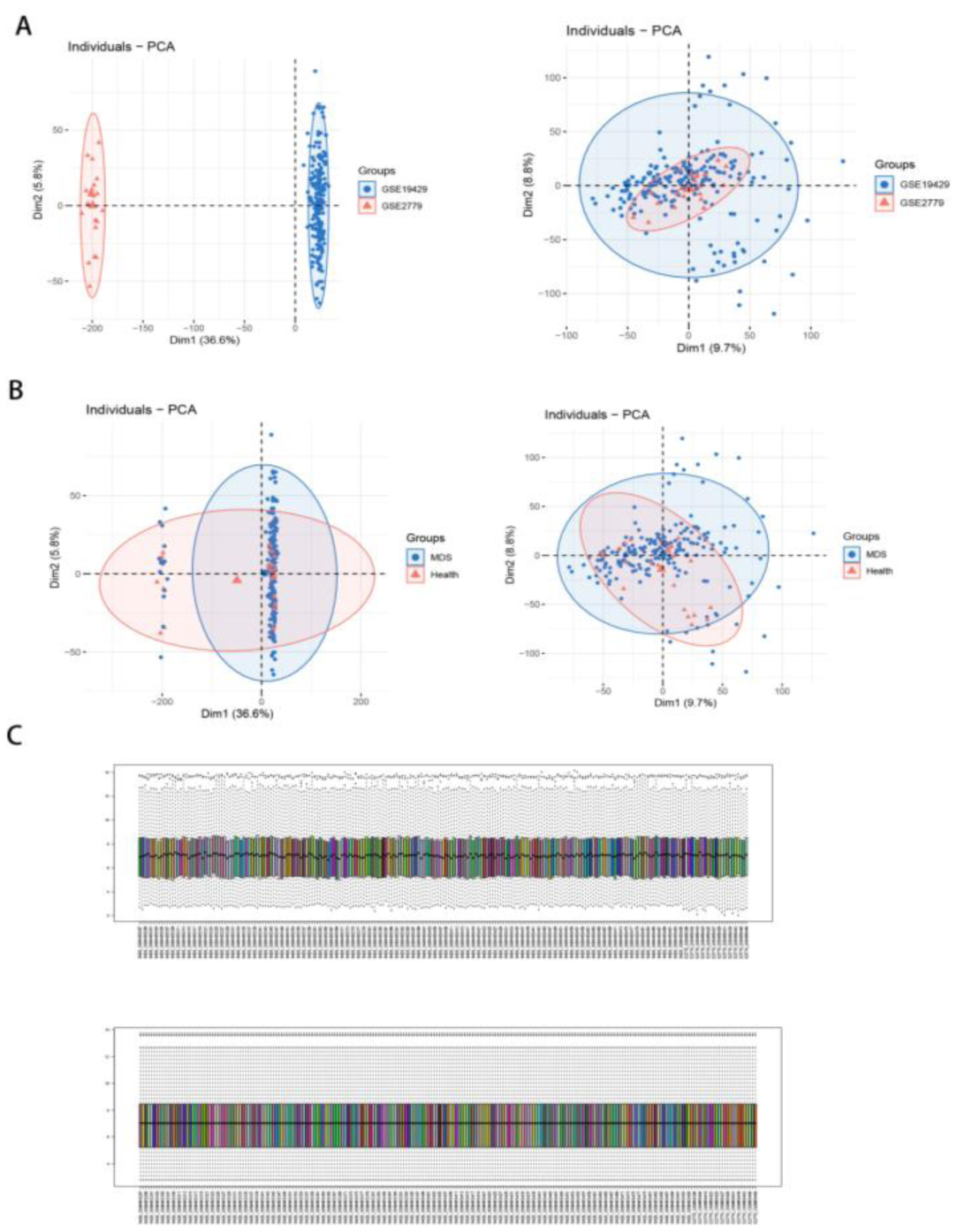
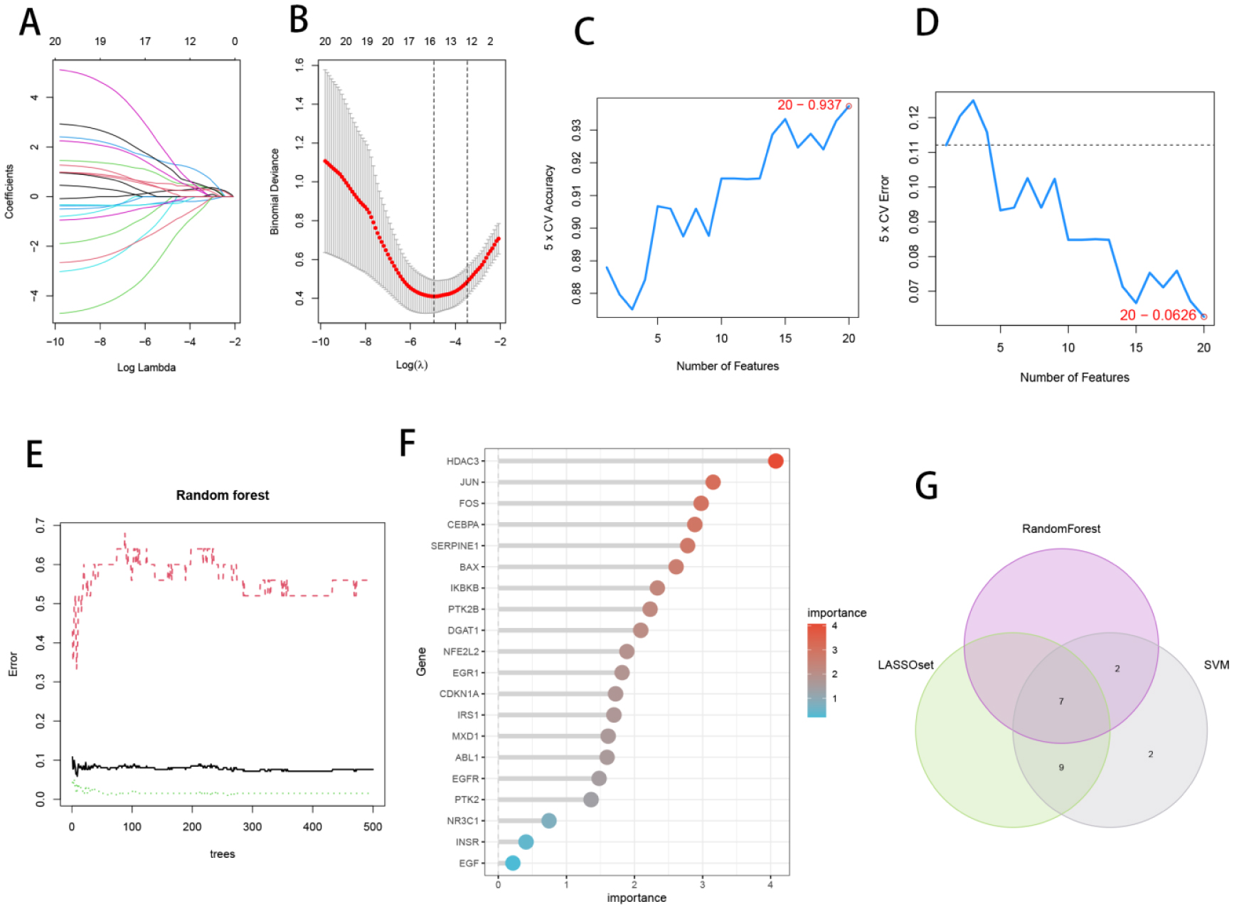
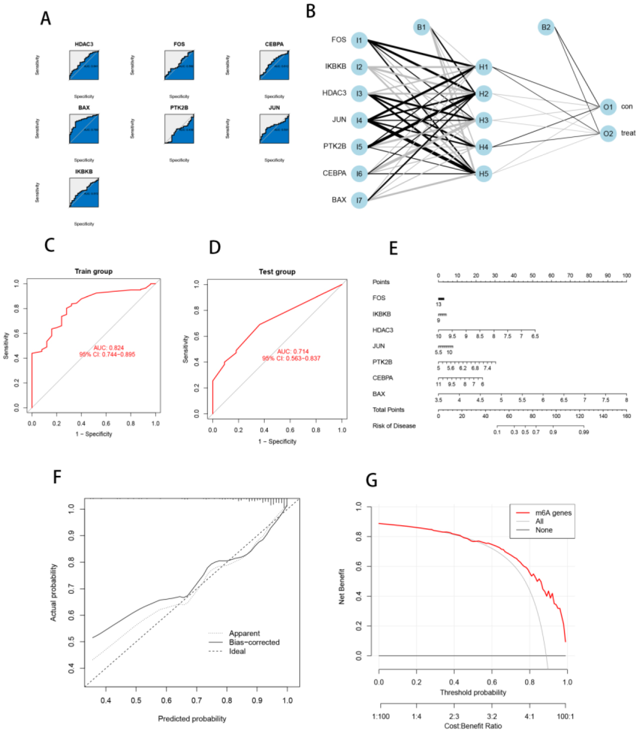
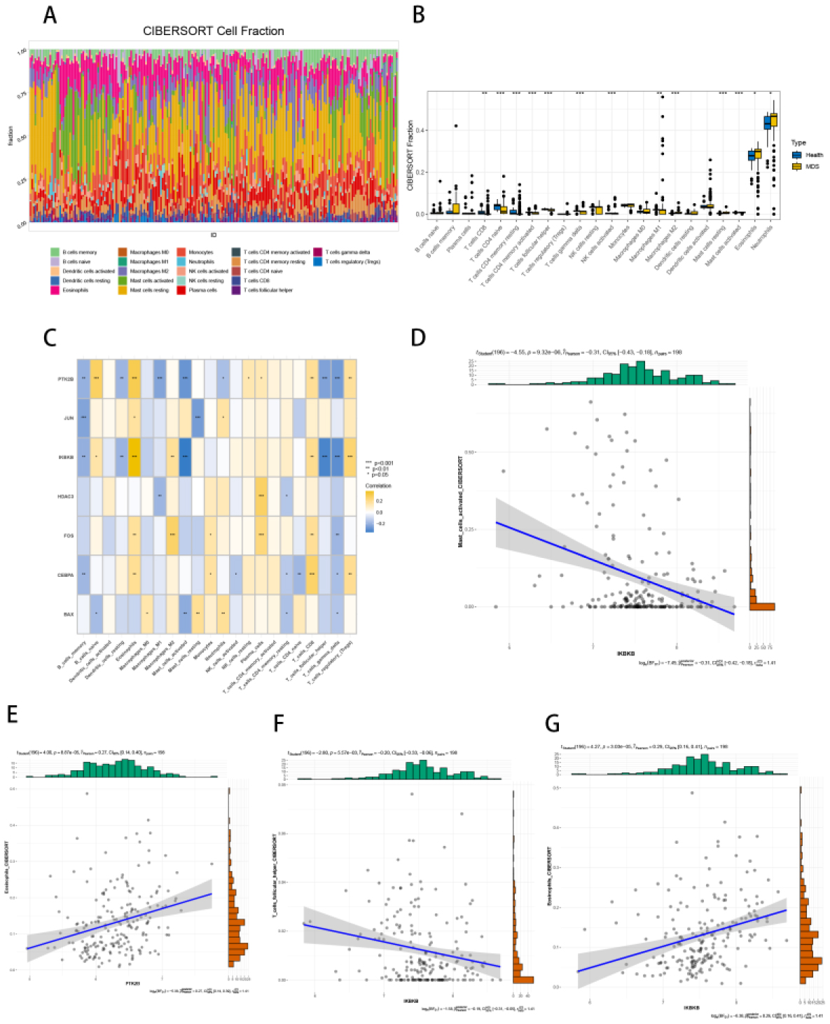
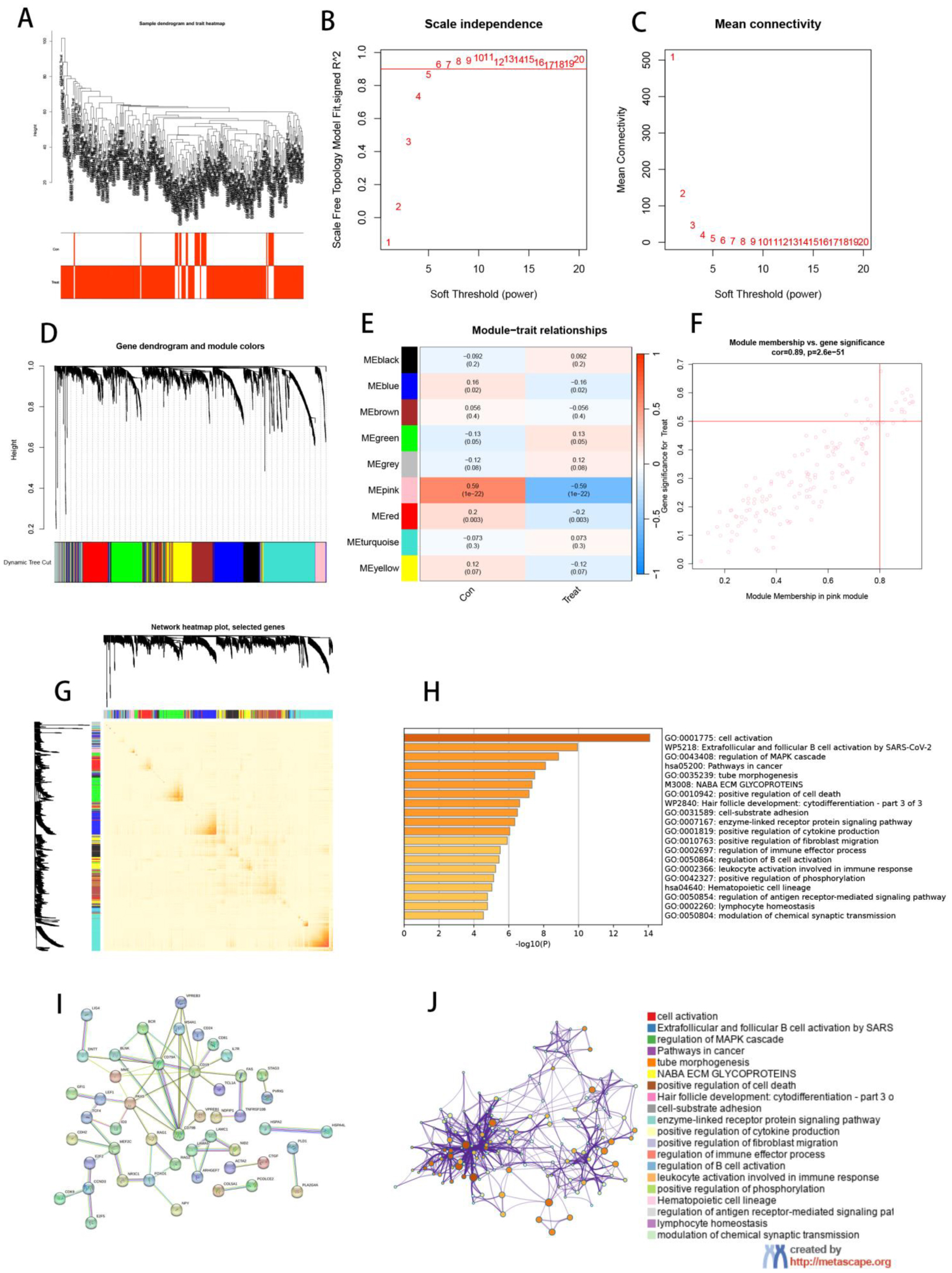
The dataset of MDS in the paper was obtained from the GEO database, and aging-related genes were taken from HAGR. Specific genes were screened by three machine learning algorithms. Then, artificial neural network (ANN) models and Nomogram models were developed to validate the effectiveness of the methods. Finally, aging subtypes were established, and the correlation between MDS and the immune microenvironment was analyzed using bioinformatics analysis tools. Weighted correlation network analysis (WGCNA) and single cell analysis were also added to validate the consistency of the result analysis.
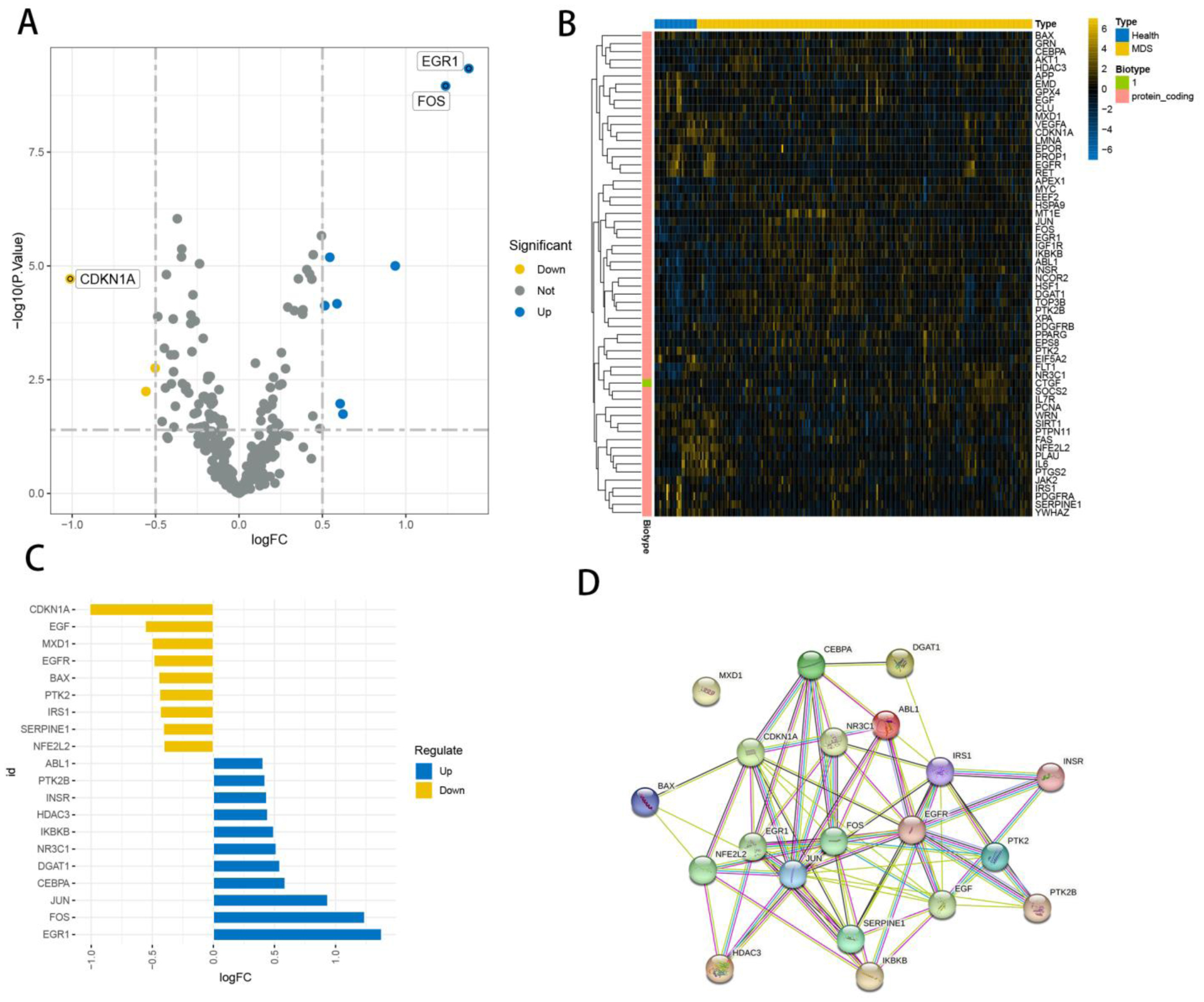
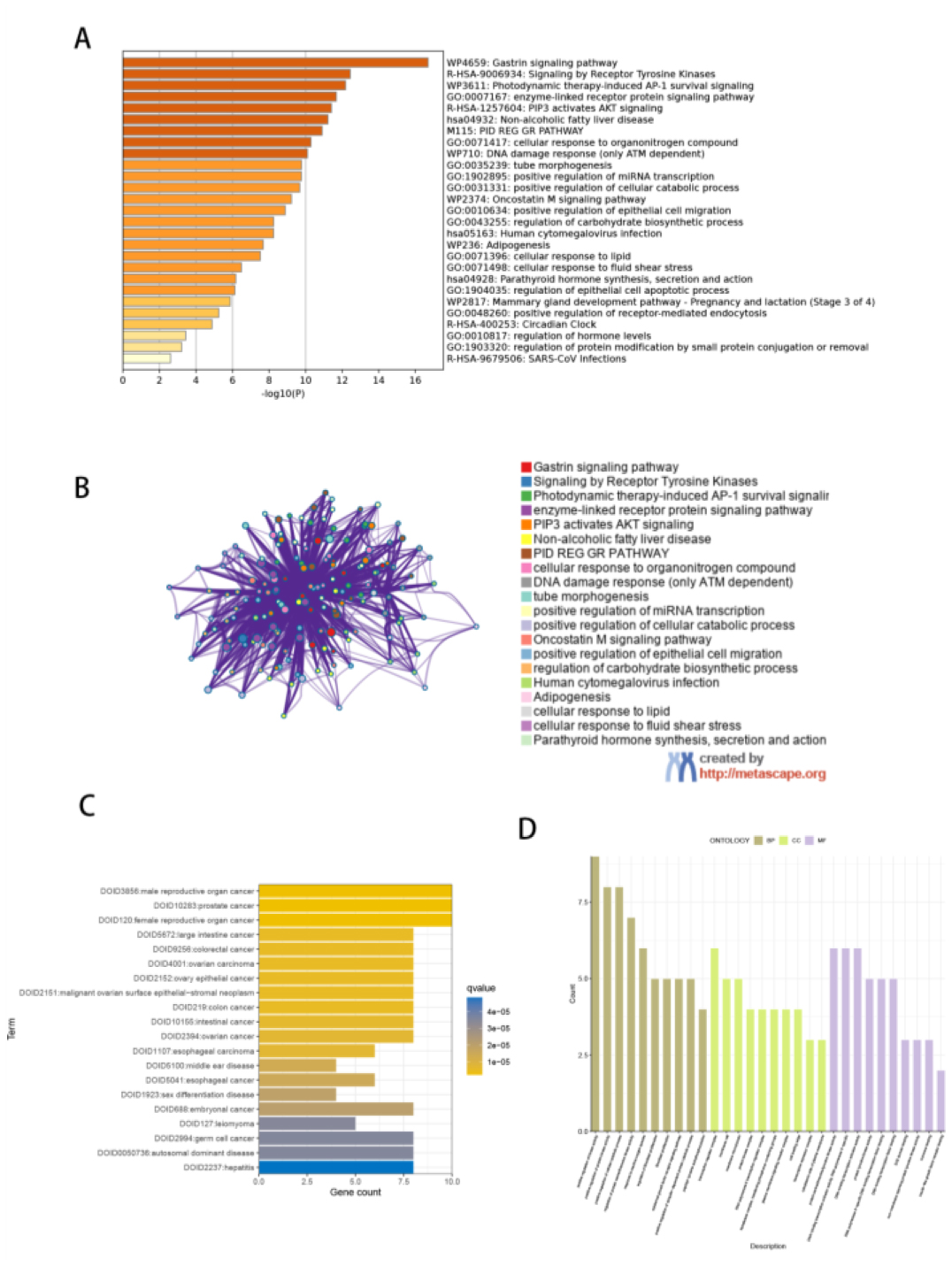
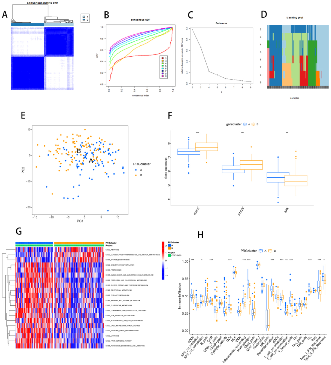
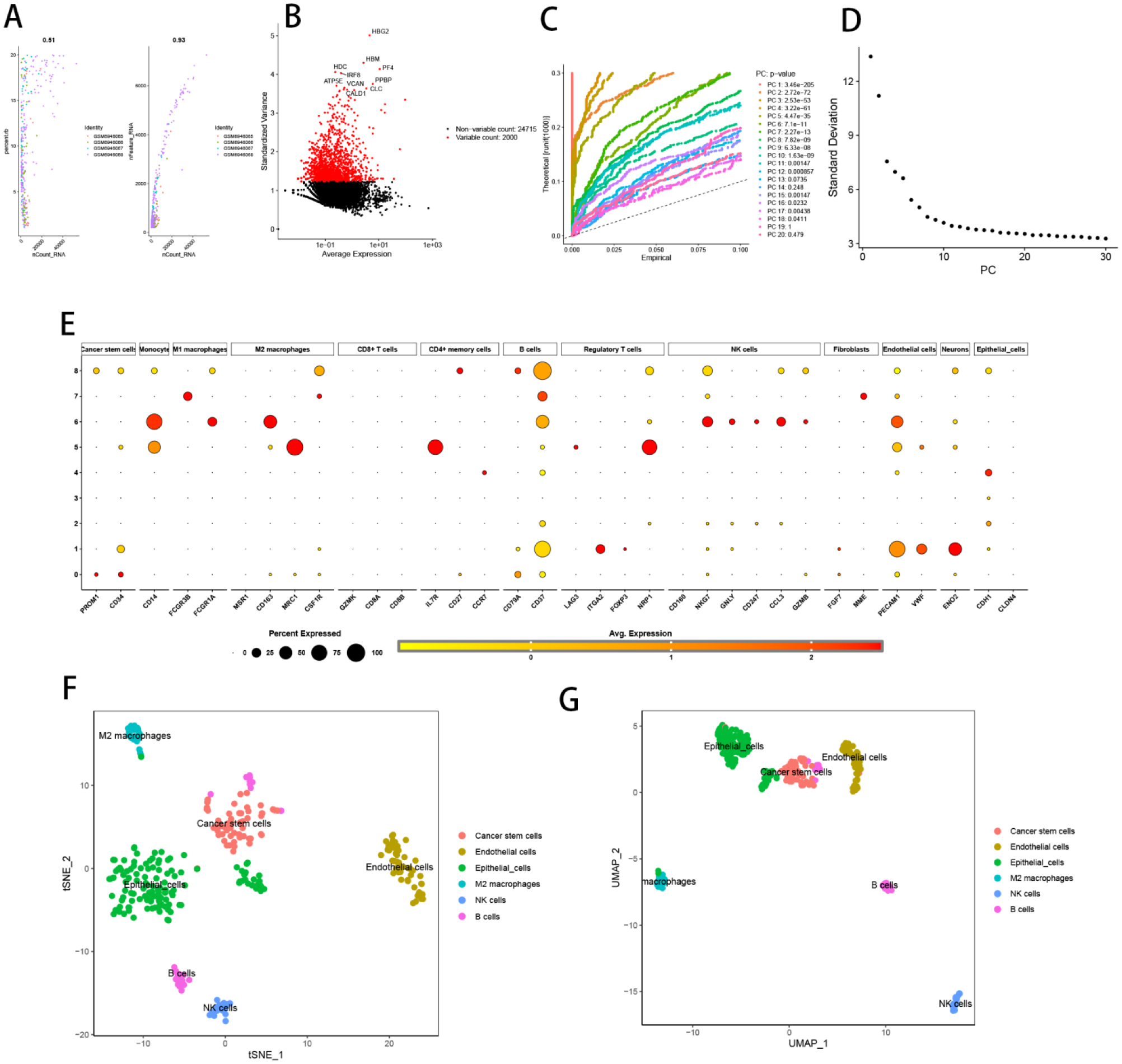
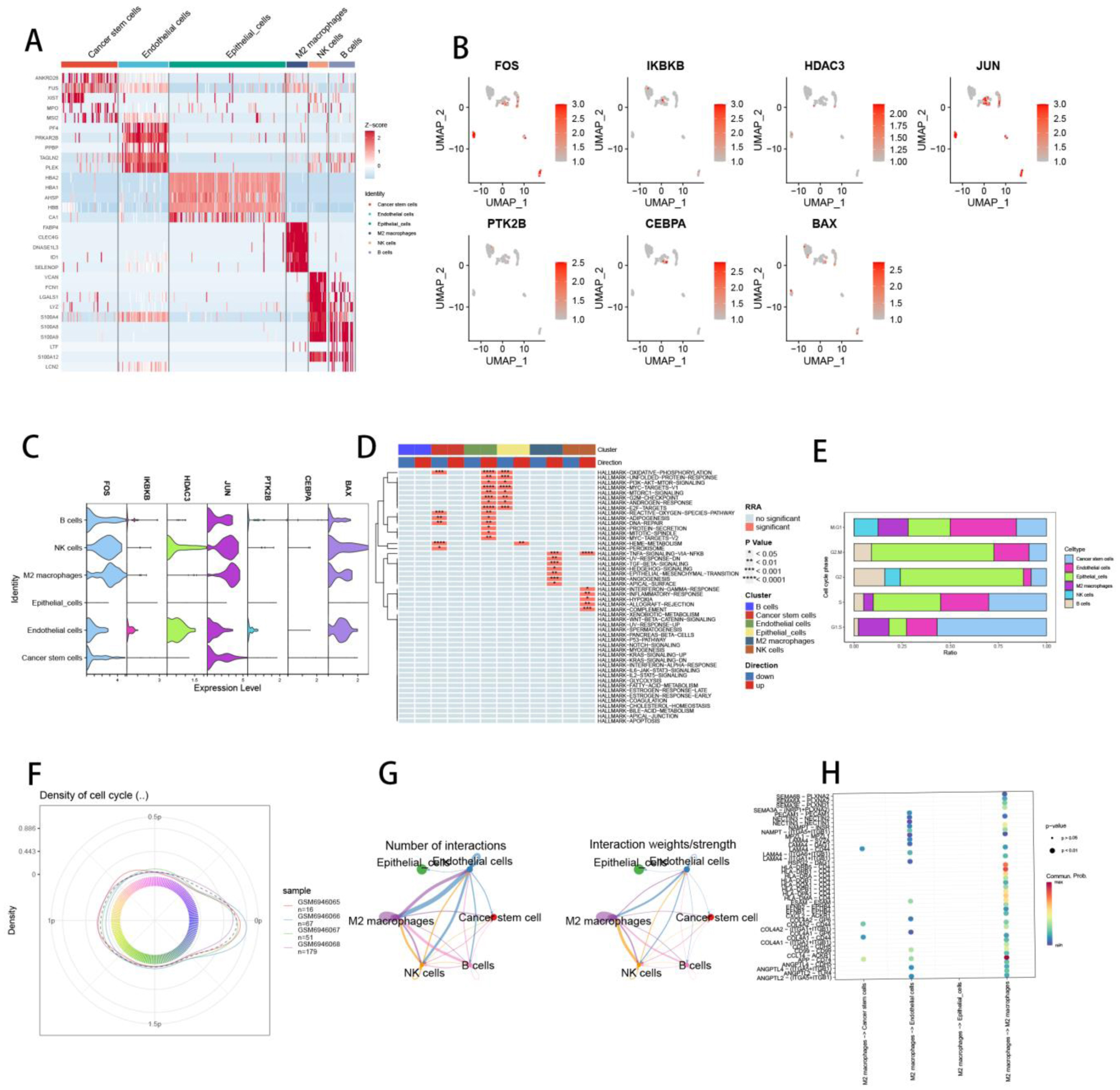
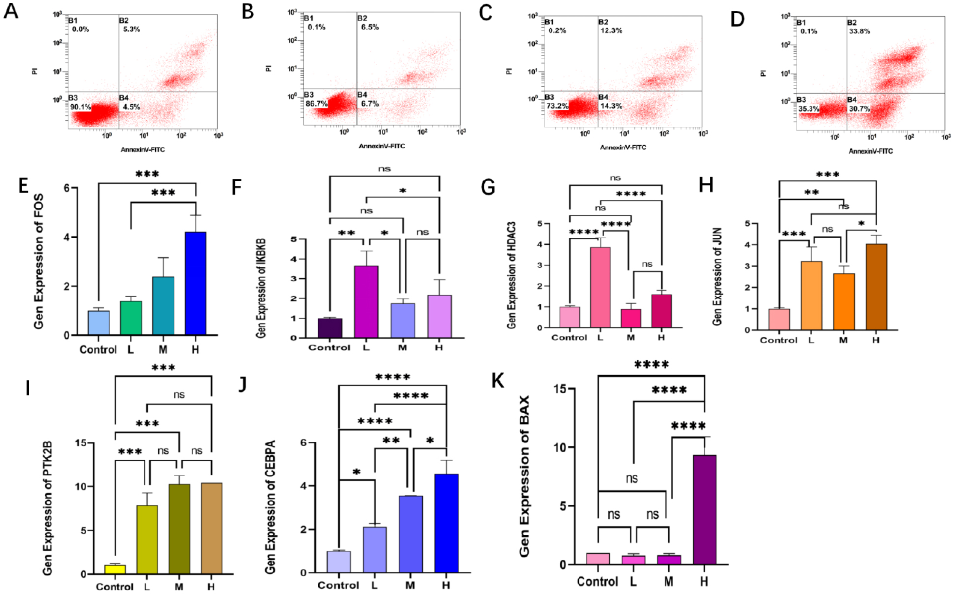
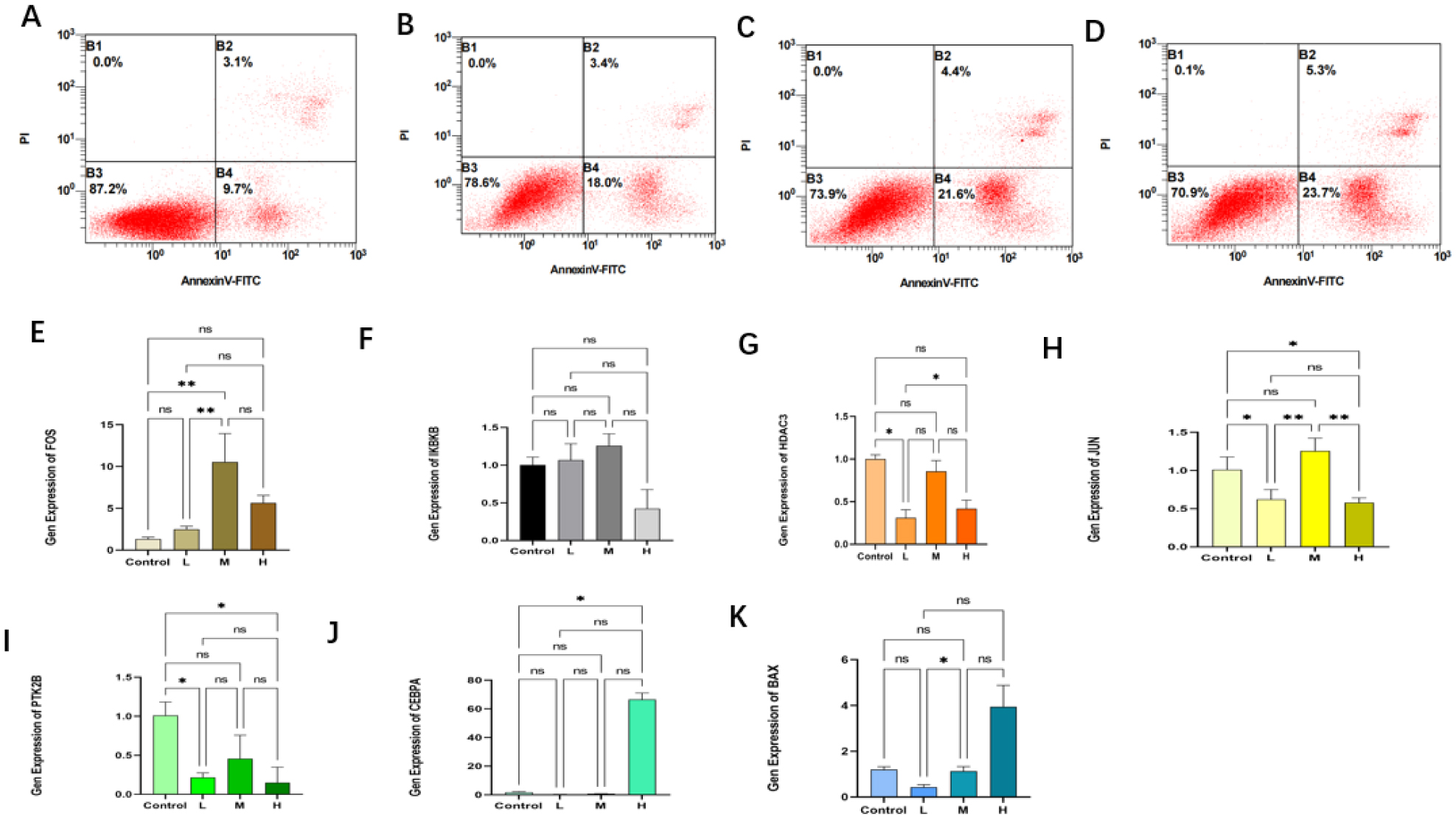
Seven core genes associated with ARG were screened by differential analysis, enrichment analysis and machine learning algorithms for accurate diagnosis of MDS. Subsequently, two subtypes of senescent expressions were identified based on ARG, illustrating that different subtypes have different biological and immune functions. The cell clustering results obtained from manual annotation were validated using single cell analysis, and the expression of 7 pivotal genes in MDS was verified by flow cytometry and RT-PCR.
The findings demonstrate a key role of senescence in the immunological milieu of MDS, giving new insights into MDS pathogenesis and potential treatments. The findings also show that aging plays an important function in the immunological microenvironment of MDS, giving new insights into the pathogenesis of MDS and possible immunotherapy.
Citation: Xiao-Li Gu, Li Yu, Yu Du, Xiu-Peng Yang, Yong-Gang Xu. Identification and validation of aging-related genes and their classification models based on myelodysplastic syndromes[J]. AIMS Bioengineering, 2023, 10(4): 440-465. doi: 10.3934/bioeng.2023026
Myelodysplastic syndrome is a malignant clonal disorder of hematopoietic stem cells (HSC) with both myelodysplastic problems and hematopoietic disorders. The greatest risk factor for the development of MDS is advanced age, and aging causes dysregulation and decreased function of the immune and hematopoietic systems. However, the mechanisms by which this occurs remain to be explored. Therefore, we explore the association between MDS and aging genes through a classification model and use bioinformatics analysis tools to explore the relationship between MDS aging subtypes and the immune microenvironment.
The dataset of MDS in the paper was obtained from the GEO database, and aging-related genes were taken from HAGR. Specific genes were screened by three machine learning algorithms. Then, artificial neural network (ANN) models and Nomogram models were developed to validate the effectiveness of the methods. Finally, aging subtypes were established, and the correlation between MDS and the immune microenvironment was analyzed using bioinformatics analysis tools. Weighted correlation network analysis (WGCNA) and single cell analysis were also added to validate the consistency of the result analysis.
Seven core genes associated with ARG were screened by differential analysis, enrichment analysis and machine learning algorithms for accurate diagnosis of MDS. Subsequently, two subtypes of senescent expressions were identified based on ARG, illustrating that different subtypes have different biological and immune functions. The cell clustering results obtained from manual annotation were validated using single cell analysis, and the expression of 7 pivotal genes in MDS was verified by flow cytometry and RT-PCR.
The findings demonstrate a key role of senescence in the immunological milieu of MDS, giving new insights into MDS pathogenesis and potential treatments. The findings also show that aging plays an important function in the immunological microenvironment of MDS, giving new insights into the pathogenesis of MDS and possible immunotherapy.

| [1] |
Sekeres MA, Taylor J (2022) Diagnosis and treatment of myelodysplastic syndromes: a review. Jama 328: 872-880. https://doi.org/10.1001/jama.2022.14578 
|
| [2] |
Trowbridge JJ, Starczynowski DT (2021) Innate immune pathways and inflammation in hematopoietic aging, clonal hematopoiesis, and MDS. J Exp Med 218: e20201544. https://doi.org/10.1084/jem.20201544
|
| [3] |
López-Otín C, Blasco MA, Partridge L, et al. (2013) The hallmarks of aging. Cell 153: 1194-1217. https://doi.org/10.1016/j.cell.2013.05.039
|
| [4] |
Steensma DP, Bejar R, Jaiswal S, et al. (2015) Clonal hematopoiesis of indeterminate potential and its distinction from myelodysplastic syndromes. Blood 126: 9-16. https://doi.org/10.1182/blood-2015-03-631747
|
| [5] |
Prasanna PG, Citrin DE, Hildesheim J, et al. (2021) Therapy-induced senescence: opportunities to improve anticancer therapy. JNCI 113: 1285-1298. https://doi.org/10.1093/jnci/djab064
|
| [6] |
Ogrodnik M, Evans SA, Fielder E, et al. (2021) Whole-body senescent cell clearance alleviates age-related brain inflammation and cognitive impairment in mice. Aging cell 20: e13296. https://doi.org/10.1111/acel.13296
|
| [7] |
Tian J, Bai Y, Liu A, et al. (2021) Identification of key biomarkers for thyroid cancer by integrative gene expression profiles. Exp Biol Med 246: 1617-1625. https://doi.org/10.1177/15353702211008809
|
| [8] |
Xie X, Wang EC, Xu D, et al. (2021) Bioinformatics analysis reveals the potential diagnostic biomarkers for abdominal aortic aneurysm. Front Cardiovasc Med 8: 656263. https://doi.org/10.3389/fcvm.2021.656263
|
| [9] |
Liu J, Zhou S, Li S, et al. (2019) Eleven genes associated with progression and prognosis of endometrial cancer (EC) identified by comprehensive bioinformatics analysis. Cancer Cell Int 19: 136. https://doi.org/10.1186/s12935-019-0859-1
|
| [10] |
Szklarczyk D, Franceschini A, Wyder S, et al. (2015) STRING v10: protein-protein interaction networks, integrated over the tree of life. Nucleic Acids Res 43: D447-D452. https://doi.org/10.1093/nar/gku1003
|
| [11] |
Zhou X, Du J, Liu C, et al. (2021) A pan-cancer analysis of CD161, a potential new immune checkpoint. Front Immunol 12: 688215. https://doi.org/10.3389/fimmu.2021.688215
|
| [12] |
Wang L, Wang D, Yang L, et al. (2022) Cuproptosis related genes associated with Jab1 shapes tumor microenvironment and pharmacological profile in nasopharyngeal carcinoma. Front Immunol 13: 989286. https://doi.org/10.3389/fimmu.2022.989286
|
| [13] |
Guo C, Gao YY, Ju QQ, et al. (2021) The landscape of gene co-expression modules correlating with prognostic genetic abnormalities in AML. J Transl Med 19: 228. https://doi.org/10.1186/s12967-021-02914-2
|
| [14] |
Yang L, Pan X, Zhang Y, et al. (2022) Bioinformatics analysis to screen for genes related to myocardial infarction. Front Genet 13: 990888. https://doi.org/10.3389/fgene.2022.990888
|
| [15] |
Ding L, Yu Q, Yang S, et al. (2022) Comprehensive analysis of HHLA2 as a prognostic biomarker and its association with immune infiltrates in hepatocellular carcinoma. Front Immunol 13: 831101. https://doi.org/10.3389/fimmu.2022.831101
|
| [16] |
Ranade NV, Nagarajan S, Sarvothaman V, et al. (2021) ANN based modelling of hydrodynamic cavitation processes: biomass pre-treatment and wastewater treatment. Ultrason Sonochem 72: 105428. https://doi.org/10.1016/j.ultsonch.2020.105428
|
| [17] |
Hu X, Wang J, Ju Y, et al. (2022) Combining metabolome and clinical indicators with machine learning provides some promising diagnostic markers to precisely detect smear-positive/negative pulmonary tuberculosis. BMC Infect Dis 22: 707. https://doi.org/10.1186/s12879-022-07694-8
|
| [18] |
Ning L, Wang X, Xuan B, et al. (2023) Identification and investigation of depression-related molecular subtypes in inflammatory bowel disease and the anti-inflammatory mechanisms of paroxetine. Front Immunol 14: 1145070. https://doi.org/10.3389/fimmu.2023.1145070
|
| [19] | Wang X, Wu Y, Wen D, et al. (2020) An individualized immune prognostic index is a superior predictor of survival of hepatocellular carcinoma. Med Sci Monit 26: e921786. https://doi.org/10.12659/MSM.921786 |
| [20] | Lin W, Wang Y, Chen Y, et al. (2021) Role of calcium signaling pathway-related gene regulatory networks in ischemic stroke based on multiple WGCNA and single-cell analysis. Oxid Med Cell Longev 2021: 8060477. https://doi.org/10.1155/2021/8060477 |
| [21] |
Zhuang W, Sun H, Zhang S, et al. (2021) An immunogenomic signature for molecular classification in hepatocellular carcinoma. Mol Ther Nucleic Acids 25: 105-115. https://doi.org/10.1016/j.omtn.2021.06.024
|
| [22] |
Liu K, Chen S, Lu R (2021) Identification of important genes related to ferroptosis and hypoxia in acute myocardial infarction based on WGCNA. Bioengineered 12: 7950-7963. https://doi.org/10.1080/21655979.2021.1984004
|
| [23] |
Wu X, Sui Z, Zhang H, et al. (2020) Integrated analysis of lncRNA-mediated ceRNA network in lung adenocarcinoma. Front Oncol 10: 554759. https://doi.org/10.3389/fonc.2020.554759
|
| [24] |
Korsunsky I, Millard N, Fan J, et al. (2019) Fast, sensitive and accurate integration of single-cell data with Harmony. Nat Methods 16: 1289-1296. https://doi.org/10.1038/s41592-019-0619-0
|
| [25] |
Yu L, Shen N, Shi Y, et al. (2022) Characterization of cancer-related fibroblasts (CAF) in hepatocellular carcinoma and construction of CAF-based risk signature based on single-cell RNA-seq and bulk RNA-seq data. Front Immunol 13: 1009789. https://doi.org/10.3389/fimmu.2022.1009789
|
| [26] |
Aran D, Looney AP, Liu L, et al. (2019) Reference-based analysis of lung single-cell sequencing reveals a transitional profibrotic macrophage. Nat Immunol 20: 163-172. https://doi.org/10.1038/s41590-018-0276-y
|
| [27] |
Sinha D, Kumar A, Kumar H, et al. (2018) dropClust: efficient clustering of ultra-large scRNA-seq data. Nucleic Acids Res 46: e36. https://doi.org/10.1093/nar/gky007
|
| [28] |
Zheng SC, Stein-O'Brien G, Augustin JJ, et al. (2022) Universal prediction of cell-cycle position using transfer learning. Genome Biol 23: 41. https://doi.org/10.1186/s13059-021-02581-y
|
| [29] |
Prata LGPL, Ovsyannikova IG, Tchkonia T, et al. (2018) Senescent cell clearance by the immune system: emerging therapeutic opportunities. Semin Immunol 40: 101275. https://doi.org/10.1016/j.smim.2019.04.003
|
| [30] |
López-Domínguez JA, Rodríguez-López S, Ahumada-Castro U, et al. (2021) Cdkn1a transcript variant 2 is a marker of aging and cellular senescence. Aging 13: 13380-13392. https://doi.org/10.18632/aging.203110
|
| [31] |
Kaya Z, Karan BM, Almalı N (2022) CDKN1A (p21 gene) polymorphisms correlates with age in esophageal cancer. Mol Biol Rep 49: 249-258. https://doi.org/10.1007/s11033-021-06865-1
|
| [32] |
Wu Y, Li D, Wang Y, et al. (2018) Beta-defensin 2 and 3 promote bacterial clearance of pseudomonas aeruginosa by inhibiting macrophage autophagy through downregulation of early growth response gene-1 and c-FOS. Front Immunol 9: 211. https://doi.org/10.3389/fimmu.2018.00211
|
| [33] |
Wang B, Guo H, Yu H, et al. (2021) The role of the transcription factor EGR1 in cancer. Front Oncol 11: 642547. https://doi.org/10.3389/fonc.2021.642547
|
| [34] |
Feng X, Shikama Y, Shichishima T, et al. (2013) Impairment of FOS mRNA stabilization following translation arrest in granulocytes from myelodysplastic syndrome patients. PLoS One 8: e61107. https://doi.org/10.1371/journal.pone.0061107
|
| [35] |
Schmid JA, Birbach A (2008) IκB kinase β (IKKβ/IKK2/IKBKB)—A key molecule in signaling to the transcription factor NF-κB. Cytokine Growth Factor Rev 19: 157-165. https://doi.org/10.1016/j.cytogfr.2008.01.006
|
| [36] |
Hayden MS, Ghosh S (2004) Signaling to NF-κB. Genes Dev 18: 2195-2224. https://doi.org/10.1101/gad.1228704
|
| [37] |
Perkins ND, Gilmore TD (2006) Good cop, bad cop: the different faces of NF-kappaB. Cell Death Differ 13: 759-772. https://doi.org/10.1038/sj.cdd.4401838
|
| [38] |
Nguyen HCB, Adlanmerini M, Hauck AK, et al. (2020) Dichotomous engagement of HDAC3 activity governs inflammatory responses. Nature 584: 286-290. https://doi.org/10.1038/s41586-020-2576-2
|
| [39] |
Sarkar R, Banerjee S, Amin SA, et al. (2020) Histone deacetylase 3 (HDAC3) inhibitors as anticancer agents: a review. Eur J Med Chem 192: 112171. https://doi.org/10.1016/j.ejmech.2020.112171
|
| [40] |
Meng Q, Xia Y (2011) c-Jun, at the crossroad of the signaling network. Protein Cell 2: 889-898. https://doi.org/10.1007/s13238-011-1113-3
|
| [41] |
Shaulian E (2010) AP-1--The Jun proteins: oncogenes or tumor suppressors in disguise?. Cell Signal 22: 894-899. https://doi.org/10.1016/j.cellsig.2009.12.008
|
| [42] |
Padhy B, Hayat B, Nanda GG, et al. (2017) Pseudoexfoliation and Alzheimer's associated CLU risk variant, rs2279590, lies within an enhancer element and regulates CLU, EPHX2 and PTK2B gene expression. Hum Mol Genet 26: 4519-4529. https://doi.org/10.1093/hmg/ddx329
|
| [43] |
Leroy H, Roumier C, Huyghe P, et al. (2005) CEBPA point mutations in hematological malignancies. Leukemia 19: 329-334. https://doi.org/10.1038/sj.leu.2403614
|
| [44] |
Pabst T, Mueller BU (2009) Complexity of CEBPA dysregulation in human acute myeloid leukemia. Clin Cancer Res 15: 5303-5307. https://doi.org/10.1158/1078-0432.CCR-08-2941
|
| [45] |
Spitz AZ, Gavathiotis E (2022) Physiological and pharmacological modulation of BAX. Trends Pharmacol Sci 43: 206-220. https://doi.org/10.1016/j.tips.2021.11.001
|
| [46] |
Matsuyama S, Palmer J, Bates A, et al. (2016) Bax-induced apoptosis shortens the life span of DNA repair defect Ku70-knockout mice by inducing emphysema. Exp Biol Med 241: 1265-1271. https://doi.org/10.1177/1535370216654587
|
| [47] |
Ying Z, Huang XF, Xiang X, et al. (2019) A safe and potent anti-CD19 CAR T cell therapy. Nat Med 25: 947-953. https://doi.org/10.1038/s41591-019-0421-7
|
| [48] |
Scheuermann RH, Racila E (1995) CD19 antigen in leukemia and lymphoma diagnosis and immunotherapy. Leuk Lymphoma 18: 385-397. https://doi.org/10.3109/10428199509059636
|
| [49] |
Huse K, Bai B, Hilden VI, et al. (2022) Mechanism of CD79A and CD79B support for IgM+ B cell fitness through B cell receptor surface expression. J Immunol 209: 2042-2053. https://doi.org/10.4049/jimmunol.2200144
|
| [50] |
Petersdorf EW (2017) In celebration of ruggero ceppellini: HLA in transplantation. HLA 89: 71-76. https://doi.org/10.1111/tan.12955
|
| [51] |
Visentin J, Couzi L, Taupin JL (2021) Clinical relevance of donor-specific antibodies directed at HLA-C: a long road to acceptance. HLA 97: 3-14. https://doi.org/10.1111/tan.14106
|
| [52] |
Gulandris F, Bacis S, Campoli R, et al. (2021) A novel HLA-C allele, HLA-C* 14: 125. HLA 97: 375-377. https://doi.org/10.1111/tan.14192
|
| [53] |
Zhao S, Chen N, He Y, et al. (2022) The novel HLA-C allele, HLA-C*03:537 in a Chinese individual. HLA 100: 376-377. https://doi.org/10.1111/tan.14715
|
| [54] |
Popēna I, Ābols A, Saulīte L, et al. (2018) Effect of colorectal cancer-derived extracellular vesicles on the immunophenotype and cytokine secretion profile of monocytes and macrophages. Cell Commun Signal 16: 17. https://doi.org/10.1186/s12964-018-0229-y
|
| [55] |
Liu J, Wang H, Zhang L, et al. (2022) Periodontal ligament stem cells promote polarization of M2 macrophages. J Leukoc Biol 111: 1185-1197. https://doi.org/10.1002/JLB.1MA1220-853RR
|
 bioeng-10-04-026-s001.pdf bioeng-10-04-026-s001.pdf |
 |
Figures(12)

Xiao-Li Gu, Li Yu, Yu Du, Xiu-Peng Yang, Yong-Gang Xu. Identification and validation of aging-related genes and their classification models based on myelodysplastic syndromes[J]. AIMS Bioengineering, 2023, 10(4): 440-465. doi: 10.3934/bioeng.2023026


 DownLoad: