Accounting for the Trump factor in modeling the COVID-19 epidemic: the case of Louisiana

Antonio N. Bojanic; Antonio N. Bojanic

doi:10.3934/bdia.2021006

Big Data and Information Analytics

2021, Volume 6, 74-85. doi: 10.3934/bdia.2021006

Previous Article Next Article

Research article

Accounting for the Trump factor in modeling the COVID-19 epidemic: the case of Louisiana

Antonio N. Bojanic ^,

Department of Economics, Tulane University, Charles Avenue New Orleans, LA, USA

Received: 21 January 2021 Accepted: 30 June 2021 Published: 05 July 2021

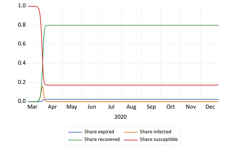
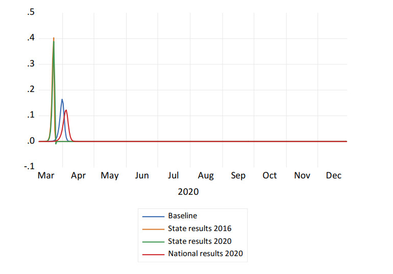
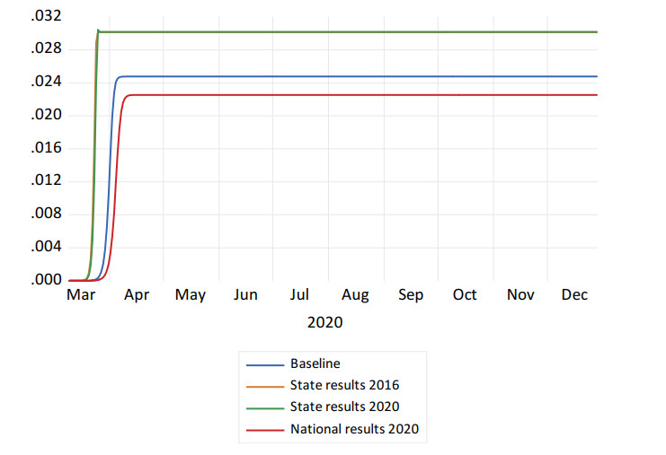
Utilizing a SIRE model, I analyze the impact of the 'Trump factor', defined as the ratio of Republican to Democratic voters, in the spread of COVID-19 in the state of Louisiana. The principal findings are these: when the Trump factor is estimated with 2016 State election results, the share of infections peaks at around 40 percent, and the share of expired (deaths) plateaus at around 3.015 percent of the state's population. Utilizing 2020 State election data, the share of infections decreases slightly – to 39 percent – and the share of expired plateaus at 3.018 percent. If the Trump factor is measured utilizing 2020 National election results, the share of infections in Louisiana would only reach 12 percent of the population and the share of expired would stabilize at 2.254 percent, reflecting a decrease in the number of total deaths of roughly 23, 459 individuals. An important conclusion is that had Trump shown more interest, and relied more heavily, on the advice of his health experts to make public pronouncements about the pandemic, perhaps the evolution of the virus in the US would not have been as tragic and costly as it has been.
- COVID-19,
- SIRE model,
- Trump factor,
- Louisiana
Citation: Antonio N. Bojanic. Accounting for the Trump factor in modeling the COVID-19 epidemic: the case of Louisiana[J]. Big Data and Information Analytics, 2021, 6: 74-85. doi: 10.3934/bdia.2021006

Related Papers:

Abstract

Utilizing a SIRE model, I analyze the impact of the 'Trump factor', defined as the ratio of Republican to Democratic voters, in the spread of COVID-19 in the state of Louisiana. The principal findings are these: when the Trump factor is estimated with 2016 State election results, the share of infections peaks at around 40 percent, and the share of expired (deaths) plateaus at around 3.015 percent of the state's population. Utilizing 2020 State election data, the share of infections decreases slightly – to 39 percent – and the share of expired plateaus at 3.018 percent. If the Trump factor is measured utilizing 2020 National election results, the share of infections in Louisiana would only reach 12 percent of the population and the share of expired would stabilize at 2.254 percent, reflecting a decrease in the number of total deaths of roughly 23, 459 individuals. An important conclusion is that had Trump shown more interest, and relied more heavily, on the advice of his health experts to make public pronouncements about the pandemic, perhaps the evolution of the virus in the US would not have been as tragic and costly as it has been.

References

[1]	National Research Council, Committee on Population, (2013), Public Health and Medical Care Systems, In: US health in international perspective: Shorter lives, poorer health, Washington: National Academies Press.
[2]	Kermack WO, McKendrick AG, (1927) A contribution to the mathematical theory of epidemics. Proc R Soc Lond 115: 700-721.
[3]	Tollefson J, (2020) How Trump damaged science—and why it could take decades to recover. Nature 586: 190-194. doi: 10.1038/d41586-020-02800-9
[4]	Thrush G, 'It affects virtually nobody, ' Trump says, minimizing the effect of the coronavirus on young people as the U.S. death toll hits 200,000. New York Times, 2020.
[5]	Nayer Z, Community outbreaks of Covid-19 often emerge after Trump's campaign rallies. Stat News, 2020.
[6]	Waldrop T, Emily G, The White House Coronavirus Cluster Is a Result of the Trump Administration's Policies, 2020. Available from: https://www.americanprogress.org/issues/healthcare/news/2020/10/16/491695/white-house-coronavirus-cluster-result-trump-administrations-policies/.
[7]	Carlisle M, Three weeks after Trump's Tulsa rally, Oklahoma reports record high COVID-19 numbers. Time, 2020.
[8]	Paz C, All the President's Lies About the Coronavirus. The Atlantic, 2020.
[9]	Hahn RA, (2021) Estimating the COVID-related deaths attributable to president Trump's early pronouncements about masks. Int J Health Serv 51: 14-17. doi: 10.1177/0020731420960345
[10]	Bernheim BD, Buchmann N, Freitas-Groff Z, et al., The Effects of Large Group Meetings on the Spread of COVID-19: The Case of Trump Rallies, Available from: https://siepr.stanford.edu/research/publications/effects-large-group-meetings-spread-covid-19-case-trump-rallies.
[11]	Dave DM, Friedson AI, Matsuzawa K, Risk aversion, offsetting community effects, and covid-19: Evidence from an indoor political rally, 2020. Available from: https://www.nber.org/papers/w27522.
[12]	Niburski K, Niburski O, (2020) Impact of Trump's promotion of unproven COVID-19 treatments and subsequent internet trends: observational study. J Med Internet Res 22: e20044.
[13]	Boynton MH, O'Hara RE, Tennen H, et al. (2020) The impact of public health organization and political figure message sources on reactions to coronavirus prevention messages. Am J Prev Med 60: 136-138.
[14]	Evanega S, Lynas M, Adams J, et al. (2020) Coronavirus Misinformation: Quantifying Sources and Themes in the COVID-19 'infodemic'. JMIR Preprints, 19.
[15]	Tassier T, (2013) The Economics of Epidemiology, Springer-Verlag Berlin Heidelberg.
[16]	Rossen LM, Branum AM, Ahmad FB, et al. (2020) Excess deaths associated with COVID-19, by age and race and ethnicity—United States, January 26-October 3, 2020. Morb Mortal Wkly Rep, 69: 1522-1527. doi: 10.15585/mmwr.mm6942e2

Reader Comments

Your name:*

Email:*
© 2021 the Author(s), licensee AIMS Press. This is an open access article distributed under the terms of the Creative Commons Attribution License (http://creativecommons.org/licenses/by/4.0)