A volatile trading pattern on a given day in a financial market presents an opportunity for traders to maximize the difference between their buying and selling prices. In order to formulate trading strategies it may be advantageous to study typical trading patterns. This paper first describes how clustering can be used to profile typical volatile trading patterns. Fuzzy c-means provides a better description of individual trading patterns, since they can display certain aspects of different trading profiles. While daily volatility profile is a useful indicator for trading a stock, the volatility history is also an important part of the decision making process. This paper further proposes a fuzzy temporal meta-clustering algorithm that not only captures the daily volatility but also puts it in a historical perspective by including the volatility of previous two weeks in the meta-profile.
Citation: Pawan Lingras, Farhana Haider, Matt Triff. Fuzzy temporal meta-clustering of financial trading volatility patterns[J]. Big Data and Information Analytics, 2017, 2(3): 219-238. doi: 10.3934/bdia.2017018
[1] | Guojun Gan, Qiujun Lan, Shiyang Sima . Scalable Clustering by Truncated Fuzzy c-means. Big Data and Information Analytics, 2016, 1(2): 247-259. doi: 10.3934/bdia.2016007 |
[2] | Marco Tosato, Jianhong Wu . An application of PART to the Football Manager data for players clusters analyses to inform club team formation. Big Data and Information Analytics, 2018, 3(1): 43-54. doi: 10.3934/bdia.2018002 |
[3] | Yaguang Huangfu, Guanqing Liang, Jiannong Cao . MatrixMap: Programming abstraction and implementation of matrix computation for big data analytics. Big Data and Information Analytics, 2016, 1(4): 349-376. doi: 10.3934/bdia.2016015 |
[4] | Jinyuan Zhang, Aimin Zhou, Guixu Zhang, Hu Zhang . A clustering based mate selection for evolutionary optimization. Big Data and Information Analytics, 2017, 2(1): 77-85. doi: 10.3934/bdia.2017010 |
[5] | Robin Cohen, Alan Tsang, Krishna Vaidyanathan, Haotian Zhang . Analyzing opinion dynamics in online social networks. Big Data and Information Analytics, 2016, 1(4): 279-298. doi: 10.3934/bdia.2016011 |
[6] | Xing Tan, Giri Kumar Tayi . CERTONTO: TOWARDS AN ONTOLOGICAL REPRESENTATION OF FAIR TRADE CERTIFICATION STANDARDS. Big Data and Information Analytics, 2017, 2(3&4): 255-264. doi: 10.3934/bdia.2017022 |
[7] | Guojun Gan, Kun Chen . A Soft Subspace Clustering Algorithm with Log-Transformed Distances. Big Data and Information Analytics, 2016, 1(1): 93-109. doi: 10.3934/bdia.2016.1.93 |
[8] | Ming Yang, Dunren Che, Wen Liu, Zhao Kang, Chong Peng, Mingqing Xiao, Qiang Cheng . On identifiability of 3-tensors of multilinear rank (1; Lr; Lr). Big Data and Information Analytics, 2016, 1(4): 391-401. doi: 10.3934/bdia.2016017 |
[9] | Ruiqi Li, Yifan Chen, Xiang Zhao, Yanli Hu, Weidong Xiao . TIME SERIES BASED URBAN AIR QUALITY PREDICATION. Big Data and Information Analytics, 2016, 1(2): 171-183. doi: 10.3934/bdia.2016003 |
[10] | Subrata Dasgupta . Disentangling data, information and knowledge. Big Data and Information Analytics, 2016, 1(4): 377-390. doi: 10.3934/bdia.2016016 |
A volatile trading pattern on a given day in a financial market presents an opportunity for traders to maximize the difference between their buying and selling prices. In order to formulate trading strategies it may be advantageous to study typical trading patterns. This paper first describes how clustering can be used to profile typical volatile trading patterns. Fuzzy c-means provides a better description of individual trading patterns, since they can display certain aspects of different trading profiles. While daily volatility profile is a useful indicator for trading a stock, the volatility history is also an important part of the decision making process. This paper further proposes a fuzzy temporal meta-clustering algorithm that not only captures the daily volatility but also puts it in a historical perspective by including the volatility of previous two weeks in the meta-profile.
A financial trader finds a daily price pattern interesting when it is volatile. The higher the fluctuations in prices, the more volatile the pattern. In order to manage a large number of patterns, it will be necessary to group these patterns based on the extent of volatility. We can segment daily patterns based on values of the Black Scholes index. This segmentation is essentially a clustering of one dimensional representation (Black Scholes index) of the daily pattern. Black Scholes index is a single concise index to identify volatility in a daily pattern. However, a complete distribution of prices during the day can provide more elaborate information on the volatility during the day. While a distribution consisting of the frequency of different prices is not a concise description for a single day, it can be a very useful representation of daily patterns for clustering based on volatility. Clustering is one of the frequently used unsupervised data mining techniques for grouping similar objects. In conventional crisp clustering schemes, an object is assigned to one and only one cluster. There is no room for ambiguity in such a clustering. Fuzzy
Finally, the paper proposes a fuzzy extension of a novel recursive approach to temporal clustering in a granular environment. In a granular temporal environment a daily pattern is connected to historical and future daily patterns. Traditionally, clustering of granules is done in isolation without any information on the clustering of the connected granules. Such a clustering will only allow us to create the profile of a stock based on daily volatility. However, a trader will typically want to know how long the stock has been volatile to figure out where the stock is in terms of its volatility cycle. The proposed fuzzy extension of a recursive temporal meta-clustering algorithm enhances the representation of a daily pattern with the clustering information of the daily patterns of the same stock from recent history. The clustering of such an enhanced representation is iterative. Each iteration uses the results of previous clustering of historical temporal patterns until a stable clustering of all the patterns is achieved. These repeated applications of clustering are called meta-clustering because we use clustering information from previous iterations to modify the representation of the granules. The resulting meta-profiles augment the daily volatility profile with historical volatility for the same financial instrument.
Volatility of Financial Data Series is an important indicator used by traders. The fluctuation in prices create trading opportunities. Volatility is a measure for variation of price of a financial instrument over time. Black Scholes index of volatility can be a good way to measure this. The equation of volatility index is an extension from the Nobel prize winning Black Scholes model which estimates the price of an option over time. This model is widely used by options market participants. The key idea behind the model is to hedge the option by buying and selling the underlying asset in just the right way and, as a consequence, to eliminate risk. The instantaneous log returns of the stock price considered in this formula is an infinitesimal random walk with drift, or more precisely is a geometric Brownian motion. The equation to estimate volatility using this model is:
Volatility=√LogPriceRelativeVariance×(Observations−1), | (1) |
where
Our data set contains average prices at 10 minute intervals of 223 instruments transacted on 121 days comprising a total of 27,012 records. Each daily pattern has 39 intervals. This data set is used to create two representations of the daily patterns. The first representation is a five dimensional pattern, which represents 10, 25, 50, 75 and 90 percentile values of the prices. The prices are normalized by the opening price so that a commodity selling for $100 has the same pattern as the one that is selling for $10. The five percentiles values for a sample pattern are shown in Table 1. The second representation is the one dimensional Black Scholes volatility for the day.
Percentile | 10% | 25% | 50% | 75% | 90% |
Percentile of avgp (avgpPerc) | 0.9841346 | 0.9873798 | 0.9927885 | 0.9951923 | 0.9966346 |
This section reviews conventional clustering with the popular algorithm
After the assignment of all the objects to various clusters, the new centroid vectors of the clusters are calculated as:
→ci=∑→xl∈→ci→xl∣→ci∣, where 1≤i≤k. |
Here
The quality of clustering is an important issue in the application of clustering techniques to real world data. A good measure of cluster quality will help in deciding the various parameters used in clustering algorithms. One potential parameter that is common to most clustering algorithms is the number of clusters. Several cluster validity indices have been proposed to evaluate cluster quality obtained by different clustering algorithms. An excellent summary of various validity measures can be found in Halkidi, et al. [9]. Many of the cluster validity measures are functions of the sum of within-cluster scatter to between-cluster separation. The scatter within the
Si=1∣→ci∣∑→x∈→cidistance(→x,→ci) | (2) |
dij=distance(→ci,→cj) | (3) |
where
We can sum up the scatter within cluster for all the clusters in a clustering scheme
S(C)=k∑i=1Si | (4) |
Similarly, between-cluster distance for a clustering scheme for a clustering scheme can be summed as:
D(C)=k∑i=1k∑j=1dij | (5) |
It is advisable to plot both of these measures for the datasets under study. Usually, the scatter within clusters starts rising rapidly, while distance between clusters starts falling rapidly when the number of clusters falls below a certain value. The knee of the curves can be used as the range for determining an appropriate number of clusters. We will demonstrate this process for all the datasets used in this study.
Conventional clustering assigns various objects to precisely one cluster. A fuzzy generalization of the clustering uses a fuzzy membership function to describe the degree of membership (ranging from 0 to 1) of an object to a given cluster. There is a stipulation that the sum of the fuzzy memberships of an object to all the clusters must be equal to 1.
The algorithm was first proposed by Dunn in 1973 [5]. Subsequently, a modification was proposed by Bezdek in 1981 [1]. Fuzzy
n∑i=1k∑j=1umij d(→xi,→cj) , 1<m<∞ | (6) |
where
The degree of membership given by a matrix
k∑j=1 uij = 1 ∀i | (7) |
The centroid of a fuzzy cluster is the weighted average of all objects, where the weights of each object is its degree of membership to a cluster:
→cj = ∑ni=1 umij →xi∑ni=1umij | (8) |
FCM is an iterative algorithm that terminates if
max(|ut+1ij−utij|)<δ | (9) |
where
This section describes the experiments that group daily patterns based on the Black Scholes index and percentile value representation of daily trading patterns using crisp and fuzzy clustering.
Since identifying the optimal clustering scheme is an NP hard problem, we use clustering algorithms such as
Optimal number of clusters is another significant measure in determining an appropriate clustering scheme. We used a two stage process that included first plotting the scatter within clusters. Our aim is to create as few clusters as possible without grouping heterogeneous/dissimilar objects. The scatter within clusters increases as we reduce the number of clusters. In our case, the increase is modest until the number of clusters reaches nine. The rate of increase before the number of clusters reaches nine is plotted in Fig. 1. One can clearly see the knee of a curve between two to nine clusters. The second stage involves the use of Davies-Bouldin (DB) index that minimizes the scatter within clusters and maximizes separation between clusters to the knee of the curve, i.e number of clusters between two to seven. The plot of Davies-Bouldin (DB) index is shown in Fig. 2. The goal is to select the number of clusters corresponding to the lowest DB index within the knee of the curve of the cluster scatter. Based on these two criteria, we chose five as a reasonable number of clusters.
In many cases, the groups generated by a clustering process have an implicit ordering. For example, clusters of customers in a retail store could be ordered based on their average spending and loyalty (their propensity to visit). Or products could be ordered based on their revenues, profits, and popularity (how many customers buy it). Similarly, the clusters of financial instruments (such as stocks) could be ordered based on their volatility. The volatility is an important indicator. A volatile daily pattern in a stock makes it more interesting to an aggressive trader and less interesting to a conservative trader.
Once we have obtained our clusters using the two representations, we can study the patterns and number the clusters based on their increasing volatility as shown in Fig. 4. Let
Fig. 4 shows that both the Black Scholes index and percentile value separate the clusters in a more or less similar fashion. For example, the difference between volatility increases as the ranks increase. The difference between ranks 1 and 2 is much smaller than that between ranks 4 and 5. While Black Scholes index is concise, the clustering based on percentile values show the volatility in a little more descriptive fashion without overloading the reader with too much information. The lower volatility ranks seem to have linear curve, while the higher volatility ranks seem to be parabolic or quadratic. This detailed distribution suggests that the 90th percentile prices in the most volatile cluster may be approximately 3 times the lowest prices on that day. Such information can be useful to the traders in order to decide the target prices for buying and selling, which is not available with Black and Scholes index.
Cluster number | 1 | 2 | 3 | 4 | 5 |
Percentile values | 14125 | 8676 | 3349 | 817 | 45 |
Black Scholes | 14182 | 8990 | 3061 | 684 | 95 |
cdvr1 | cdvr2 | cdvr3 | cdvr4 | cdvr5 | |
cpr1 | 10430 | 3104 | 519 | 67 | 5 |
cpr2 | 3411 | 4047 | 1089 | 123 | 6 |
cpr3 | 339 | 1727 | 1047 | 223 | 13 |
cpr4 | 2 | 112 | 404 | 258 | 41 |
cpr5 | 0 | 0 | 2 | 13 | 30 |
While the percentile values provide a more descriptive grouping of the daily trading patterns, they lack an important feature provided by the Black Scholes index, i.e. quantification of degree of volatility. In the next section, we will study the fuzzy
In the previous section, we discussed crisp clustering of daily trading patterns as a more descriptive way to categorize daily volatility than a single Black Scholes index. As discussed before, the crisp clustering forces a daily pattern into exactly one level of volatility. This is somewhat rigid compared to the continuous scale offered by the Black Scholes index. In this section, we will apply the fuzzy
Let
avgRank(xi)=k∑j=1uij×j, | (10) |
where
Instead of assigning a daily pattern to a single cluster, the fuzzy
Day:Instrument | Avg Rank | |||||
2011-08-16:3_1 | 0.04 | 0.06 | 0.09 | 0.35 | 0.46 | 4.14 |
2011-08-17:3_1 | 0.85 | 0.13 | 0.03 | 0 | 0 | 1.19 |
: | ||||||
2012-01-31:3_1 | 0.06 | 0.16 | 0.65 | 0.12 | 0.01 | 2.86 |
: | ||||||
2011-08-16:Z_2 | 0.97 | 0.03 | 0.01 | 0 | 0 | 1.04 |
: | ||||||
2012-01-31:Z_2 | 0.93 | 0.05 | 0.01 | 0 | 0 | 1.09 |
Comparison of the centroids from crisp clustering for both percentile value distribution and Black Scholes index in Fig. 3 with those obtained from fuzzy clustering in Fig. 5 suggests that fuzzy clustering tends to have more evenly distributed separation of clusters. As discussed earlier, well separated clusters is an important aspect of cluster quality measurement. The evenly distributed centroids in fuzzy clustering are possible because an object can belong to multiple clusters with different membership instead of creating an extremely volatile cluster.
The average daily patterns for each cluster shown in Fig. 5 provide a more descriptive representation of the different volatility ranks similar to the crisp clustering percentile value patterns. On the other hand, the average volatility rank given by Eq.10 provide a more concise value of the volatility similar to the Black Scholes index. Therefore, we can conclude that the average volatility rank along with the fuzzy centroids combines the best of both worlds in terms of semantics and conciseness.
In this section, we compared the segmentation of Black Scholes volatility index and two clustering alternatives of more descriptive percentile values of the daily price distribution. The fuzzy
Normally data miners consider rows to be the objects and columns as the attributes of these objects. A good example of such a dataset is a document collection or corpus. Each row in the table corresponds to a document. Each column corresponds to a keyword. We can say that this is a dataset consisting of documents represented by frequency of different keywords in the document given by the rows in the table. However, one can easily transpose this view and say that it is a collection of keywords that shows how often the keyword occurs in various documents in the collection given by the columns in the table. Information retrieval practitioners use clustering to group both documents and keywords. Slonim and Tishby [23] proposed a two stage clustering method for this application. In the first step, the keywords were grouped based on the their frequency in various documents. The documents were then represented using the clusters of keywords as opposed to individual keywords. El-Yaniv and Sourojon [6] extended this two stage approach with an iterative version where the resulting document clustering could be used to re-cluster the words and the process would continue. More generically, double clustering can be viewed as a dimensionality reduction technique that replaces the columns by groups of columns. Castellano et al. [4] further generalized double clustering using fuzzy set theory. Caruana et al. [3] showed that the use of meta-clustering, meaning clusters of clusters, can make it easier for the users to see more meaningful groupings. Ramirez et al. [21] took meta-clustering to three levels for grouping players in a game based on three different criteria: skills, preferences while playing the game, and relationships with other players. The generalization of meta-clustering can be found when bi-clustering, first introduced by Mirkin [19], was extended to tri-clustering and then more generally to n-clustering [7,8,11,12].
Lingras et al. [15] described how a granular hierarchy can be clustered iteratively with the help of static information and the dynamically changing profiles of customers and products throughout the meta-clustering process. This approach unified the conventional static clustering with the simultaneous meta-clustering such as double clustering using granular computing. Similar interdependency can also be observed in a networked environment, where objects such as phone users are connected to other phone users within the same dataset. In such a case, the profile of a phone user should include the profiles of other users created by the same clustering process. These dependencies are applicable to any social network, Lingras and Rathinavel [13] proposed a recursive clustering technique for such networked environments.
Such a recursive meta-clustering can be used with any crisp or soft clustering algorithm. The type of clustering will determine how the dynamic portion is computed. For example, for crisp clustering we will use the frequency of granules in each cluster. For fuzzy clustering, the average memberships of granules in each cluster will make up the dynamic portion. Lingras and Triff [14] compared recursive profiles obtained from both crisp and fuzzy meta-clustering. The flexible cluster memberships provided by fuzzy clustering are shown to provide more moderate and uniformly distributed clustering schemes. Recently, Lingras and Haider [16] proposed a temporal extension of the meta-clustering algorithm based on crisp clustering. As the comparison of crisp and fuzzy clustering in the previous section suggests, fuzzy clustering of percentile value patterns may be able to provide a better profiling of volatility in a daily trading pattern. Therefore, the remaining paper describes a fuzzy extension of the temporal meta-clustering algorithm that will help us put the volatility in a historical perspective.
As described by [15,17,22,24], objects are represented by both static and dynamic parts. The static part contains the attributes representing information obtained from the database. The static part does not change throughout the meta-clustering process. The dynamic part contains clustering information about the other connected objects and is derived from the previous clustering of all the objects, and changes with each iteration of the meta-clustering process. At the beginning of the clustering process, we do not have any information from a previous clustering iteration. Therefore, the dynamic part is empty and the first clustering of objects is based only on the static part. This clustering is used to produce the dynamic part containing the cluster membership information of the connected objects. Next the static and dynamic parts are concatenated and clustered. This process of clustering with the two concatenated parts and updating the dynamic part after each iteration continues as long as every two consecutive dynamic portions of clusters are divergent. The overall process is shown as a flowchart in Fig. 6.
The algorithm for the proposed recursive temporal meta-clustering is represented in Fig 7. The primary objective of the temporal meta-clustering is to recursively provide a historical perspective of the clustering. For example, let us consider daily patterns of a number of stocks that are being traded in a financial market. We want to create a measure of volatility of a daily pattern using clustering. However, profiling a stock only on one day's daily price pattern will not tell the trader if the stock is in an early or late stage of an unusual interest in the market. Therefore, we want to use volatility profiles of the recent history of a stock for creating the volatility profile of the stock on a given day. However, these historical volatility profiles require the clustering of the stock's pattern for the recent days in the same clustering algorithm leading to a recursive profiling.
The two key steps in the algorithm are creation of the static and dynamic parts. A daily pattern of a stock is naturally connected to the daily patterns of the same stock from previous days. It is fair to assume that sustained activity in a stock does not last for more than two weeks (ten trading days). Based on this assumption, we can create a graph where each daily pattern is connected to the daily patterns of the same stock from the previous ten days. That means the representation of a daily pattern has data from that day (obtained statically from the database). This static part consists of five percentile values (10%, 25%, 50%, 75%, 90%) as described in the data processing section. The historical volatility of the same stock over last ten trading days constitutes the dynamic part of the representation of a daily pattern. More specifically, the dynamic part will use the volatility ranking of the last ten trading days for the same stock based on meta-clustering information. In order to have ten days of history available in the representation of a daily pattern, our dataset consists of patterns starting from
The attribute values are weighted to ensure that the small values of the static part are not dominated by the large values of the dynamic part and vice versa. Examples of the static parts of some of the daily patterns are shown in Table 5.
Day:Instrument | p10 | p25 | p50 | p75 | p90 |
2011-08-16:3_1 | 0 | 0.28 | 0.56 | 0.67 | 0.78 |
2011-08-17:3_1 | 0 | 0 | 0.04 | 0.09 | 0.11 |
: | |||||
2012-01-31:3_1 | 0 | 0 | 0.15 | 0.29 | 0.46 |
: | |||||
2011-08-16:Z_2 | 0 | 0.027 | 0.045 | 0.05 | 0.05 |
: | |||||
2012-01-31:Z_2 | 0 | 0.01 | 0.019 | 0.03 | 0.11 |
In order to create the first dynamic part, we cluster the daily patterns using these static parts. The resulting five clusters are ranked based on their volatility. The higher values in the 90th percentile tend to suggest higher volatility. The cluster with the lowest volatility is ranked 1, the cluster with the next lowest valued centroids is ranked 2 and so on. Ranked clusters with centroid values of the percentiles from the static part are shown in Table 6.
Centers | ||||||
Rank | Cluster | p10 | p25 | p50 | p75 | p90 |
1 | C2 | 0 | 0.02 | 0.03 | 0.06 | 0.08 |
2 | C5 | 0 | 0.05 | 0.10 | 0.16 | 0.21 |
3 | C4 | 0 | 0.09 | 0.19 | 0.28 | 0.35 |
4 | C1 | 0 | 0.16 | 0.35 | 0.48 | 0.57 |
5 | C3 | 0 | 0.30 | 0.66 | 0.88 | 1.00 |
The dynamic part of a daily pattern is created by assuming that the daily pattern is related to the last ten daily patterns for the same stock. We use the last ten average volatility rankings for the same stock calculated using Eq.10 to make up the dynamic part of the representation of the daily pattern. The dynamic part puts the volatility of a stock in historical perspective. Examples of dynamic parts created after first clustering with static parts for some of the daily patterns is shown in Table 7.
Daym+1:Instrument | dm-9 | dm-8 | dm-7 | dm-6 | dm-5 | dm-4 | dm-3 | dm-2 | dm-1 | d m |
2011-08-16:3_1 | 2.69 | 2.69 | 2.70 | 2.70 | 2.69 | 2.70 | 2.68 | 2.70 | 2.70 | 2.69 |
2011-08-17:3_1 | 2.69 | 2.70 | 2.70 | 2.69 | 2.70 | 2.68 | 2.70 | 2.70 | 2.69 | 4.14 |
: | ||||||||||
2012-01-31:3_1 | 1.07 | 2.10 | 3.78 | 1.25 | 1.81 | 3.58 | 4.06 | 1.09 | 1.42 | 3.56 |
: | ||||||||||
2011-08-16:Z_2 | 2.69 | 2.70 | 2.70 | 2.70 | 2.70 | 2.70 | 2.70 | 2.70 | 2.70 | 2.69 |
: | ||||||||||
2012-01-31:Z_2 | 1.09 | 2.90 | 2.89 | 1.15 | 3.04 | 1.87 | 2.00 | 3.01 | 2.05 | 1.71 |
Static and dynamic parts of Table 5 and Table 7 are concatenated as Table 8 for the next step of the clustering. The concatenated profile with 15 attributes (5 percentiles and ranks of the last 10 days) are clustered. The resultant cluster profile is shown in Table 9. After every clustering, the dynamic part is updated and the clustering is repeated until the dynamic part converges or until the maximum number of iterations is reached.
SP | DP | ||||||||||||||
Day:Instrument | p10 | p25 | p50 | p75 | p90 | dm-9 | dm-8 | dm-7 | dm-6 | dm-5 | dm-4 | dm-3 | dm-2 | dm-1 | dm |
2011-08-16:3_1 | 0 | 0.28 | 0.56 | 0.67 | 0.78 | 2.69 | 2.69 | 2.70 | 2.70 | 2.69 | 2.70 | 2.68 | 2.70 | 2.70 | 2.70 |
2011-08-17:3_1 | 0 | 0 | 0.04 | 0.09 | 0.11 | 2.69 | 2.70 | 2.70 | 2.69 | 2.70 | 2.68 | 2.70 | 2.70 | 2.69 | 4.14 |
: | |||||||||||||||
2012-01-31:3_1 | 0 | 0 | 0.15 | 0.29 | 0.46 | 1.07 | 2.10 | 3.78 | 1.25 | 1.81 | 3.58 | 4.06 | 1.09 | 1.42 | 3.56 |
: | |||||||||||||||
2011-08-16:Z_2 | 0 | 0.03 | 0.045 | 0.05 | 0.05 | 2.69 | 2.70 | 2.70 | 2.70 | 2.70 | 2.70 | 2.70 | 2.70 | 2.70 | 2.69 |
: | |||||||||||||||
2012-01-31:Z_2 | 0 | 0.01 | 0.02 | 0.03 | 0.11 | 1.09 | 2.90 | 2.89 | 1.15 | 3.04 | 1.87 | 2.00 | 3.01 | 2.05 | 1.71 |
SP | DP | |||||||||||||||
Rank | Cluster | p10 | p25 | p50 | p75 | p90 | dm-9 | dm-8 | dm-7 | dm-6 | dm-5 | dm-4 | dm-3 | dm-2 | dm-1 | dm |
1 | C5 | 0 | 0.0530 | 0.1123 | 0.1720 | 0.2227 | 1.9925 | 1.9849 | 1.9812 | 1.9698 | 1.9645 | 1.9569 | 1.9539 | 1.9481 | 1.9409 | 1.9376 |
2 | C2 | 0 | 0.0531 | 0.1124 | 0.1721 | 0.2227 | 1.9933 | 1.9857 | 1.9820 | 1.9706 | 1.9653 | 1.9576 | 1.9546 | 1.9488 | 1.9415 | 1.9382 |
3 | C4 | 0 | 0.0531 | 0.1124 | 0.1721 | 0.2228 | 1.9937 | 1.9861 | 1.9824 | 1.9710 | 1.9657 | 1.9581 | 1.9550 | 1.9492 | 1.9419 | 1.9386 |
4 | C1 | 0 | 0.0531 | 0.1124 | 0.1722 | 0.2229 | 1.9943 | 1.9867 | 1.9830 | 1.9716 | 1.9663 | 1.9587 | 1.9556 | 1.9498 | 1.9424 | 1.9391 |
5 | C3 | 0 | 0.0532 | 0.1124 | 0.1722 | 0.2229 | 1.9946 | 1.9871 | 1.9834 | 1.9720 | 1.9666 | 1.9590 | 1.9559 | 1.9501 | 1.9427 | 1.9393 |
The recursive temporal meta-clustering process was executed for a maximum of 65 iterations. The rounded values of the dynamic parts were compared to test the convergence. After 23 iterations the result stabilized.
The final cluster centroids and their ranks obtained at iteration 23 are shown in Table 10 and Fig. 8. It is interesting to note that the average ranks in the dynamic part match the ranks of the clusters inferred from the volatility in the percentile values. That means the static and dynamic parts in the fuzzy centroids are consistent with each other.
Rank | Cluster | p10 | p25 | p50 | p75 | p90 | dm-9 | dm-8 | dm-7 | dm-6 | dm-5 | dm-4 | dm-3 | dm-2 | dm-1 | dm |
1 | C2 | 0 | 0.04 | 0.08 | 0.12 | 0.15 | 1.20 | 1.17 | 1.14 | 1.12 | 1.11 | 1.10 | 1.10 | 1.11 | 1.13 | 1.15 |
2 | C4 | 0 | 0.05 | 0.10 | 0.15 | 0.19 | 2.24 | 2.20 | 2.16 | 2.14 | 2.11 | 2.10 | 2.10 | 2.11 | 2.12 | 2.14 |
3 | C3 | 0 | 0.05 | 0.10 | 0.16 | 0.21 | 3.04 | 3.03 | 3.03 | 3.03 | 3.02 | 3.02 | 3.02 | 3.02 | 3.03 | 3.03 |
4 | C1 | 0 | 0.05 | 0.11 | 0.17 | 0.22 | 3.82 | 3.86 | 3.89 | 3.92 | 3.94 | 3.95 | 3.97 | 3.98 | 3.99 | 3.99 |
5 | C5 | 0 | 0.07 | 0.14 | 0.21 | 0.27 | 4.70 | 4.75 | 4.78 | 4.81 | 4.83 | 4.84 | 4.83 | 4.82 | 4.79 | 4.76 |
To put the volatility in historical perspective and allow traders to look at stocks differently leading to a more informed decision, we can also provide a graphical representation of a stock over previous two weeks. Figs. 9-14 show a number of different variations in the volatility of different stocks over a two-week trading period. We can analyze the activity and possible trading implications as follows:
● Stock Z_2 on 2012-01-02 shown in Fig. 9 jumped to the volatility of 5 with a steady increase in volatility from almost 2 to 5 over previous ten trading days. This stock is of high and increasing interest by the market at this time. A potential candidate for short term trading.
● Stock 3_1 on 2011-10-03 shown in Fig. 10 settled to the lowest volatility of 1 after slight turbulence over previous ten trading days. This stock is of little interest at this time.
● Stock A_10 on 2011-12-06 shown in Fig. 11 settled to the volatility of 2 after slightly higher volatility over previous ten trading days. This stock is of modest interest and will be a relatively safe trade.
● Stock 3_1 on 2011-08-16 shown in Fig. 12 settled to the volatility of 3 after slightly higher volatility over previous ten trading days. This stock is of a reasonable interest and will be potentially good trade.
● Stock A_10 on 2012-01-04 shown in Fig. 13 suddenly jumped back to the volatility of 4 after showing a decline in volatility over previous ten trading days. This stock had peaked interest of the market, but subsequently the interest waned due to lack of news, and now it has become very interesting.
● Stock A_113 on 2011-11-01 shown in Fig. 14 jumped to the volatility of 5 after hovering between 4.7 and 4.8 for previous ten trading days. The interest in this stock was percolating in anticipation of some news, and now it has become very interesting.
The historical analysis and trading implications described above use fuzzy temporal meta-clustering and would not be possible if the stocks were analyzed by studying the daily patterns in isolation.
The primary objective of the proposed meta-clustering algorithm is to generate semantically more meaningful profiles based on connections between granules. It is necessary to strike a balance between reliable and useful profiles versus computational efficiency. The proposed meta-clustering algorithm has inherent opportunities for parallel processing. Therefore, while it will require significant computational resources, they can be distributed among multiple processors resulting in a reasonable chronological time requirement. In this section, we discuss the computational requirements and describe how the algorithm can be parallelized. The implementation of parallel meta-clustering is a separate research topic in itself, and is being investigated as part of our ongoing research.
The problem of obtaining an optimal clustering scheme is NP-hard. Let us assume that there are
It is possible that if the cluster quality measure is carefully chosen, it may be possible to optimize it without having to consider all possible clustering schemes. For example, the fuzzy
The proposed meta-clustering algorithm uses multiple applications of a conventional clustering algorithm such as the
1. Apply fuzzy
2. The creation of dynamic profiles involves sorting and searching lists. There are many parallel implementations of sorting and searching that can be used to facilitate faster computations.
This paper describes a number of alternatives to the Black Scholes index for measuring volatility in daily trading in a financial market. The study uses 223 financial instruments (stocks) traded over 121 days. The daily trading patterns of these stocks are segmented based on the Black Scholes index and crisp clustering using the frequency distribution of the prices in a day. The crisp clustering provides more descriptive profiles of volatility, while Black Scholes index provides a concise volatility indicator. Fuzzy
1. The fuzzy centroids of percentile values are better separated than the crisp clustering - a desirable cluster quality measure.
2. While the fuzzy centroids provide semantic description of the volatility, the average fuzzy volatility rank will be as concise an indicator of volatility as the Black Scholes index.
The paper further extends a temporal meta-clustering algorithm based on an average fuzzy volatility rank. It makes it possible to put the volatility rankings in a historical perspective, which will aid a trader in making decisions based on where the stock is in a volatility cycle.
While the data used in this study is proprietary and part of a broader study, the proposed algorithm can be applied to publicly available historical prices from such institutions as Yahoo Finance. The low, high, closing prices and trading volumes can provide an alternative representation of volatility.
The authors would like to thank Natural Sciences and Engineering Research Council (NSERC) of Canada and Saint Mary's University for their funding of this project. The authors also appreciate the contribution of data by the company involved.
[1] |
J. C. Bezdek, Pattern Recognition with Fuzzy Objective Function Algorithms, Kluwer Academic Publishers, Norwell, MA, USA, 1981. MR631231 |
[2] |
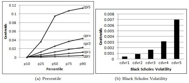
F. Black and M. Scholes, The pricing of options and corporate liabilities, The journal of political economy, 81 (1973), 637–654. doi: 10.1086/260062
![]() |
[3] |
R. Caruana, M. Elhaway, N. Nguyen and C. Smith, Meta clustering, in Data Mining, 2006. ICDM'06. Sixth International Conference on, IEEE, 2006,107–118. 10.1109/ICDM.2006.103 |
[4] | G. Castellano, A. M. Fanelli and C. Mencar, Generation of interpretable fuzzy granules by a double-clustering technique, Archives of Control Science, 12 (2002), 397–410. |
[5] |
J. C. Dunn, A fuzzy relative of the ISODATA process and its use in detecting compact well-separated clusters, Cybernetics, 3 (1973), 32–57. doi: 10.1080/01969727308546046
![]() |
[6] | R. El-Yaniv and O. Souroujon, Iterative double clustering for unsupervised and semisupervised learning, Machine Learning: ECML 2001, Springer, (2001), 121–132. |
[7] | D. Gnatyshak, D. I. Ignatov, A. Semenov and J. Poelmans, Gaining insight in social networks with biclustering and triclustering, Perspectives in Business Informatics Research, Springer, (2012), 162–171. |
[8] | D. V. Gnatyshak, D. I. Ignatov and S. O. Kuznetsov, From triadic fca to triclustering: Experimental comparison of some triclustering algorithms, CLA 2013, p249. |
[9] |
M. Halkidi, Y. Batistakis and M. Vazirgianni, Clustering validity checking methods: Part Ⅱ, ACM SIGMOD Record, 31 (2002), 19–27. doi: 10.1145/601858.601862
![]() |
[10] | J. A. Hartigan and M. A.Wong, Algorithm AS136: A K-Means Clustering Algorithm, Applied Statistics, 28 (1979), 100–108. |
[11] |
D. I. Ignatov, S. O. Kuznetsov and J. Poelmans, Concept-based biclustering for internet advertisement, in Data Mining Workshops (ICDMW), 2012 IEEE 12th International Conference on, IEEE, 2012,123–130. 10.1109/ICDMW.2012.100 |
[12] |
D. I. Ignatov, S. O. Kuznetsov, J. Poelmans and L. E. Zhukov, Can triconcepts become triclusters?, International Journal of General Systems, 42 (2013), 572–593. doi: 10.1080/03081079.2013.798899
![]() |
[13] |
P. Lingras and K. Rathinavel, Recursive Meta-clustering in a Granular Network, in Plenary talk at the Fourth International Conference of Soft Computing and Pattern Recognition, Brunei, 2012. 10.1109/ISDA.2012.6416634 |
[14] |
P. Lingras and M. Tri, Fuzzy and crisp recursive profiling of online reviewers and businesses, IEEE Transactions on Fuzzy Systems, 23 (2015), 1242–1258. doi: 10.1109/TFUZZ.2014.2349532
![]() |
[15] |
P. Lingras, A. Elagamy, A. Ammar and Z. Elouedi, Iterative meta-clustering through granular hierarchy of supermarket customers and products, Information Sciences, 257 (2014), 14–31. doi: 10.1016/j.ins.2013.09.018
![]() |
[16] | P. Lingras and F. Haider, Recursive temporal meta-clustering, Applied Soft Computing, submitted. |
[17] |
P. Lingras and K. Rathinavel, Recursive meta-clustering in a granular network, in Intelligent Systems Design and Applications (ISDA), 2012 12th International Conference on, IEEE, 2012,770–775. 10.1109/ISDA.2012.6416634 |
[18] |
J. MacQueen, Some methods for classification and analysis of multivariate observations, in Proceedings of Fifth Berkeley Symposium on Mathematical Statistics and Probability, 1 (1967), 281–297. MR0214227 |
[19] |
B. Mirkin, Mathematical Classification and Clustering, Kluwer Academic Publishers, Boston, MA, USA, 1996. MR1480413 |
[20] |
W. Pedrycz and J. Waletzky, Fuzzy clustering with partial supervision, IEEE Transactions on Systems, Man, and Cybernetics, Part B, 27 (1997), 787–795. doi: 10.1109/3477.623232
![]() |
[21] | D. Ramirez-Cano, S. Colton and R. Baumgarten, Player classification using a meta-clustering approach, in Proceedings of the 3rd Annual International Conference Computer Games, Multimedia and Allied Technology, 2010,297–304. |
[22] |
K. Rathinavel and P. Lingras, A granular recursive fuzzy meta-clustering algorithm for social networks, in IFSA World Congress and NAFIPS Annual Meeting (IFSA/NAFIPS), 2013 Joint, IEEE, 2013,567–572. 10.1109/IFSA-NAFIPS.2013.6608463 |
[23] |
N. Slonim and N. Tishby, Document clustering using word clusters via the information bottleneck method, in 23rd Annual International ACM SIGIR Conference on Research and Development in Information Retrieval, 2000,208–215. 10.1145/345508.345578 |
[24] | M. Triff and P. Lingras, Recursive profiles of businesses and reviewers on yelp. com, Rough Sets, Fuzzy Sets, Data Mining, and Granular Computing, Springer, (2013), 325–336. |
Percentile | 10% | 25% | 50% | 75% | 90% |
Percentile of avgp (avgpPerc) | 0.9841346 | 0.9873798 | 0.9927885 | 0.9951923 | 0.9966346 |
Cluster number | 1 | 2 | 3 | 4 | 5 |
Percentile values | 14125 | 8676 | 3349 | 817 | 45 |
Black Scholes | 14182 | 8990 | 3061 | 684 | 95 |
cdvr1 | cdvr2 | cdvr3 | cdvr4 | cdvr5 | |
cpr1 | 10430 | 3104 | 519 | 67 | 5 |
cpr2 | 3411 | 4047 | 1089 | 123 | 6 |
cpr3 | 339 | 1727 | 1047 | 223 | 13 |
cpr4 | 2 | 112 | 404 | 258 | 41 |
cpr5 | 0 | 0 | 2 | 13 | 30 |
Day:Instrument | Avg Rank | |||||
2011-08-16:3_1 | 0.04 | 0.06 | 0.09 | 0.35 | 0.46 | 4.14 |
2011-08-17:3_1 | 0.85 | 0.13 | 0.03 | 0 | 0 | 1.19 |
: | ||||||
2012-01-31:3_1 | 0.06 | 0.16 | 0.65 | 0.12 | 0.01 | 2.86 |
: | ||||||
2011-08-16:Z_2 | 0.97 | 0.03 | 0.01 | 0 | 0 | 1.04 |
: | ||||||
2012-01-31:Z_2 | 0.93 | 0.05 | 0.01 | 0 | 0 | 1.09 |
Day:Instrument | p10 | p25 | p50 | p75 | p90 |
2011-08-16:3_1 | 0 | 0.28 | 0.56 | 0.67 | 0.78 |
2011-08-17:3_1 | 0 | 0 | 0.04 | 0.09 | 0.11 |
: | |||||
2012-01-31:3_1 | 0 | 0 | 0.15 | 0.29 | 0.46 |
: | |||||
2011-08-16:Z_2 | 0 | 0.027 | 0.045 | 0.05 | 0.05 |
: | |||||
2012-01-31:Z_2 | 0 | 0.01 | 0.019 | 0.03 | 0.11 |
Centers | ||||||
Rank | Cluster | p10 | p25 | p50 | p75 | p90 |
1 | C2 | 0 | 0.02 | 0.03 | 0.06 | 0.08 |
2 | C5 | 0 | 0.05 | 0.10 | 0.16 | 0.21 |
3 | C4 | 0 | 0.09 | 0.19 | 0.28 | 0.35 |
4 | C1 | 0 | 0.16 | 0.35 | 0.48 | 0.57 |
5 | C3 | 0 | 0.30 | 0.66 | 0.88 | 1.00 |
Daym+1:Instrument | dm-9 | dm-8 | dm-7 | dm-6 | dm-5 | dm-4 | dm-3 | dm-2 | dm-1 | d m |
2011-08-16:3_1 | 2.69 | 2.69 | 2.70 | 2.70 | 2.69 | 2.70 | 2.68 | 2.70 | 2.70 | 2.69 |
2011-08-17:3_1 | 2.69 | 2.70 | 2.70 | 2.69 | 2.70 | 2.68 | 2.70 | 2.70 | 2.69 | 4.14 |
: | ||||||||||
2012-01-31:3_1 | 1.07 | 2.10 | 3.78 | 1.25 | 1.81 | 3.58 | 4.06 | 1.09 | 1.42 | 3.56 |
: | ||||||||||
2011-08-16:Z_2 | 2.69 | 2.70 | 2.70 | 2.70 | 2.70 | 2.70 | 2.70 | 2.70 | 2.70 | 2.69 |
: | ||||||||||
2012-01-31:Z_2 | 1.09 | 2.90 | 2.89 | 1.15 | 3.04 | 1.87 | 2.00 | 3.01 | 2.05 | 1.71 |
SP | DP | ||||||||||||||
Day:Instrument | p10 | p25 | p50 | p75 | p90 | dm-9 | dm-8 | dm-7 | dm-6 | dm-5 | dm-4 | dm-3 | dm-2 | dm-1 | dm |
2011-08-16:3_1 | 0 | 0.28 | 0.56 | 0.67 | 0.78 | 2.69 | 2.69 | 2.70 | 2.70 | 2.69 | 2.70 | 2.68 | 2.70 | 2.70 | 2.70 |
2011-08-17:3_1 | 0 | 0 | 0.04 | 0.09 | 0.11 | 2.69 | 2.70 | 2.70 | 2.69 | 2.70 | 2.68 | 2.70 | 2.70 | 2.69 | 4.14 |
: | |||||||||||||||
2012-01-31:3_1 | 0 | 0 | 0.15 | 0.29 | 0.46 | 1.07 | 2.10 | 3.78 | 1.25 | 1.81 | 3.58 | 4.06 | 1.09 | 1.42 | 3.56 |
: | |||||||||||||||
2011-08-16:Z_2 | 0 | 0.03 | 0.045 | 0.05 | 0.05 | 2.69 | 2.70 | 2.70 | 2.70 | 2.70 | 2.70 | 2.70 | 2.70 | 2.70 | 2.69 |
: | |||||||||||||||
2012-01-31:Z_2 | 0 | 0.01 | 0.02 | 0.03 | 0.11 | 1.09 | 2.90 | 2.89 | 1.15 | 3.04 | 1.87 | 2.00 | 3.01 | 2.05 | 1.71 |
SP | DP | |||||||||||||||
Rank | Cluster | p10 | p25 | p50 | p75 | p90 | dm-9 | dm-8 | dm-7 | dm-6 | dm-5 | dm-4 | dm-3 | dm-2 | dm-1 | dm |
1 | C5 | 0 | 0.0530 | 0.1123 | 0.1720 | 0.2227 | 1.9925 | 1.9849 | 1.9812 | 1.9698 | 1.9645 | 1.9569 | 1.9539 | 1.9481 | 1.9409 | 1.9376 |
2 | C2 | 0 | 0.0531 | 0.1124 | 0.1721 | 0.2227 | 1.9933 | 1.9857 | 1.9820 | 1.9706 | 1.9653 | 1.9576 | 1.9546 | 1.9488 | 1.9415 | 1.9382 |
3 | C4 | 0 | 0.0531 | 0.1124 | 0.1721 | 0.2228 | 1.9937 | 1.9861 | 1.9824 | 1.9710 | 1.9657 | 1.9581 | 1.9550 | 1.9492 | 1.9419 | 1.9386 |
4 | C1 | 0 | 0.0531 | 0.1124 | 0.1722 | 0.2229 | 1.9943 | 1.9867 | 1.9830 | 1.9716 | 1.9663 | 1.9587 | 1.9556 | 1.9498 | 1.9424 | 1.9391 |
5 | C3 | 0 | 0.0532 | 0.1124 | 0.1722 | 0.2229 | 1.9946 | 1.9871 | 1.9834 | 1.9720 | 1.9666 | 1.9590 | 1.9559 | 1.9501 | 1.9427 | 1.9393 |
Rank | Cluster | p10 | p25 | p50 | p75 | p90 | dm-9 | dm-8 | dm-7 | dm-6 | dm-5 | dm-4 | dm-3 | dm-2 | dm-1 | dm |
1 | C2 | 0 | 0.04 | 0.08 | 0.12 | 0.15 | 1.20 | 1.17 | 1.14 | 1.12 | 1.11 | 1.10 | 1.10 | 1.11 | 1.13 | 1.15 |
2 | C4 | 0 | 0.05 | 0.10 | 0.15 | 0.19 | 2.24 | 2.20 | 2.16 | 2.14 | 2.11 | 2.10 | 2.10 | 2.11 | 2.12 | 2.14 |
3 | C3 | 0 | 0.05 | 0.10 | 0.16 | 0.21 | 3.04 | 3.03 | 3.03 | 3.03 | 3.02 | 3.02 | 3.02 | 3.02 | 3.03 | 3.03 |
4 | C1 | 0 | 0.05 | 0.11 | 0.17 | 0.22 | 3.82 | 3.86 | 3.89 | 3.92 | 3.94 | 3.95 | 3.97 | 3.98 | 3.99 | 3.99 |
5 | C5 | 0 | 0.07 | 0.14 | 0.21 | 0.27 | 4.70 | 4.75 | 4.78 | 4.81 | 4.83 | 4.84 | 4.83 | 4.82 | 4.79 | 4.76 |