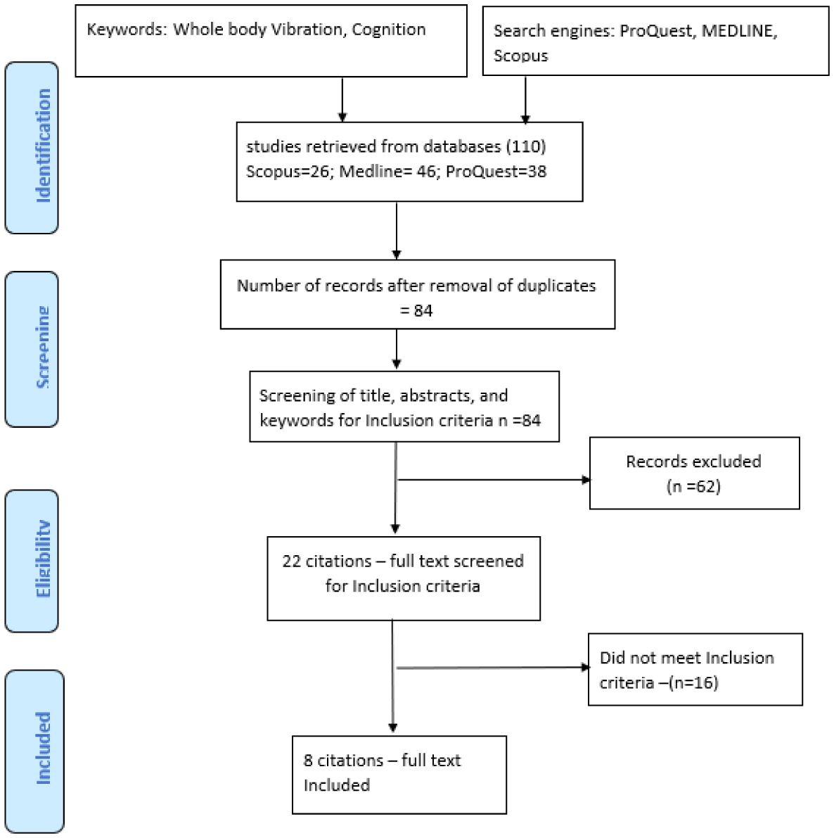
Whole Body Vibration has been found to induce physiological changes in human subjects, improving their neuromuscular, respiratory and cardiovascular functions. Evidence from animal research prove that whole-body vibration appears to induce changes in molecular and cellular levels to alter cognitive functions in mice. There is evolving evidence for a potential value of whole body vibration in improving cognition and preventing the development of age-related cognitive disorders in humans. However, literature on the biological consequences of whole-body vibration on the human brain is scanty. If so, gathering the available evidences would help decide the possibility of designing appropriate whole-body vibration protocols to extend its application to induce neurocognitive enhancement and optimize its effects. Therefore, a systematic review of the literature was performed, consulting the ProQuest, MEDLINE and Scopus bibliographic databases, to summarize the available scientific evidence on the effects of whole-body vibration on cognitive functions in adults. Results of the review suggest that whole-body vibration therapy enhances a wide spectrum of cognitive functions in adults although there isn't enough evidence available yet to be able to design a standardized protocol to achieve optimum cognitive enhancement.
Citation: Nisha Shantakumari, Musaab Ahmed. Whole body vibration therapy and cognitive functions: a systematic review[J]. AIMS Neuroscience, 2023, 10(2): 130-143. doi: 10.3934/Neuroscience.2023010
Whole Body Vibration has been found to induce physiological changes in human subjects, improving their neuromuscular, respiratory and cardiovascular functions. Evidence from animal research prove that whole-body vibration appears to induce changes in molecular and cellular levels to alter cognitive functions in mice. There is evolving evidence for a potential value of whole body vibration in improving cognition and preventing the development of age-related cognitive disorders in humans. However, literature on the biological consequences of whole-body vibration on the human brain is scanty. If so, gathering the available evidences would help decide the possibility of designing appropriate whole-body vibration protocols to extend its application to induce neurocognitive enhancement and optimize its effects. Therefore, a systematic review of the literature was performed, consulting the ProQuest, MEDLINE and Scopus bibliographic databases, to summarize the available scientific evidence on the effects of whole-body vibration on cognitive functions in adults. Results of the review suggest that whole-body vibration therapy enhances a wide spectrum of cognitive functions in adults although there isn't enough evidence available yet to be able to design a standardized protocol to achieve optimum cognitive enhancement.

| [1] |
Freitas ACS, Gaspar JF, de Souza GCRM, et al. (2022) The effects of whole-body vibration on cognition: a systematic review. J Hum Growth Dev 32: 108-119. https://doi.org/10.36311/jhgd.v32.12864 
|
| [2] |
Trans T, Aaboe J, Henriksen M, Christensen R, et al. (2009) Effect of whole-body vibration exercise on muscle strength and proprioception in females with knee osteoarthritis. Knee 16: 256-26. https://doi.org/10.1016/j.knee.2008.11.014
|
| [3] | Wysocki A, Butler M, Shamliyan T, et al. (2019) Whole-Body Vibration Therapy for Osteoporosis: State of the Science. Ann Intern Med 15: 680-686. https://doi.org/10.7326/0003-4819-155-10-201111150-00006 |
| [4] |
Zago M, Capodaglio P, Ferrario C, Tarabini M, et al. (2018) Whole-body vibration training in obese subjects: A systematic review. PLoS One 13: e0202866. https://doi.org/10.1371/journal.pone.0202866
|
| [5] |
Hillman CH, Erickson KI, Kramer AF (2008) Be smart, exercise your heart: exercise effects on brain and cognition. Nat Rev Neurosci 9: 58-65. https://doi.org/10.1038/nrn2298
|
| [6] |
Hang SS, Zhu L, Peng Y, et al. (2022) Long-term running exercise improves cognitive function and promotes microglial glucose metabolism and morphological plasticity in the hippocampus of APP/PS1 mice. J Neuroinflammation 19: 34. https://doi.org/10.1186/s12974-022-02401-5
|
| [7] |
Chan RC, Shum D, Toulopoulou T, et al. (2008) Assessment of executive functions: review of instruments and identification of critical issues. Arch Clin Neuropsychol 23: 201-16. https://doi.org/10.1016/j.acn.2007.08.010
|
| [8] | Van der Zee EA, Riedel G, Rutgers EH, et al. (2010) Enhanced neuronal activity in selective brain regions of mice induced by whole body stimulation. Fed Eur Neurosci Soc Abstr 5: 49. |
| [9] | Heesterbeek M, Jentsch M, Roemers P, et al. (2017) Whole body vibration enhances choline acetyltransferase-immunoreactivity in cortex and amygdale. J Neurol Transl Neurosci 5: 1079. |
| [10] |
Cariati I, Bonanni R, Pallone G, et al. (2022) Whole Body Vibration Improves Brain and Musculoskeletal Health by Modulating the Expression of Tissue-Specific Markers: FNDC5 as a Key Regulator of Vibration Adaptations. Int J Mol Sci 23: 10388. https://doi.org/10.3390/ijms231810388
|
| [11] |
Rosado H, Bravo J, Raimundo A, Carvalho J, et al. (2021) Effects of two 24-week multimodal exercise programs on reaction time, mobility, and dual-task performance in community-dwelling older adults at risk of falling: a randomized controlled trial. BMC Public Health 21: 408. https://doi.org/10.1186/s12889-021-10448-x
|
| [12] |
Regterschot GR, Van Heuvelen MJ, Zeinstra EB, et al. (2014) Whole body vibration improves cognition in healthy young adults. PLoS One 9: e100506. https://doi.org/10.1371/journal.pone.0100506
|
| [13] |
Boerema AS, Heesterbeek M, Boersma SA, et al. (2018) Beneficial Effects of Whole-Body Vibration on Brain Functions in Mice and Humans. Dose Response 16. https://doi.org/10.1177/1559325818811756
|
| [14] |
Paddan GS, Holmes SR, Mansfield NJ, et al. (2012) The influence of seat backrest angle on human performance during whole-body vibration. Ergonomics 55: 114-128. https://doi.org/10.1080/00140139.2011.634030
|
| [15] |
Amonette WE, Boyle M, Psarakis MB, et al. (2015) Neurocognitive responses to a single session of static squats with whole body vibration. J Strength Cond Res 29: 96-100. https://doi.org/10.1519/JSC.0b013e31829b26ce
|
| [16] |
Fereydounnia S, Shadmehr A (2020) Efficacy of whole-body vibration on neurocognitive parameters in women with and without lumbar hyper-lordosis. J Bodyw Mov Ther 24: 182-189. https://doi.org/10.1016/j.jbmt.2019.05.030
|
| [17] |
Fuermaier AB, Tucha L, Koerts J, et al. (2014) Good vibrations--effects of whole-body vibration on attention in healthy individuals and individuals with ADHD. PLoS One 9: e90747. https://doi.org/10.1371/journal.pone.0090747
|
| [18] |
Kim Ki-Hong, Lee Hyang-Beum (2018) The effects of whole body vibration exercise intervention on electroencephalogram activation and cognitive function in women with senile dementia. J Exerc Rehabil 14: 586-591. https://doi.org/10.12965/jer.1836230.115
|
| [19] |
Ghazalian F, Hakemi L, Pourkazemi L, et al. (2015) Effects of amplitudes of whole-body vibration training on left ventricular stroke volume and ejection fraction in healthy young men. Anatol J Cardiol 15: 976-80. https://doi.org/10.5152/akd.2014.5863
|
| [20] | Costantino C, Gimigliano R, Olvirri S, et al. (2014) Whole body vibration in sport: A critical review. J Sports Med Phys Fitness 54: 757-764. |
| [21] | Signorile J (2011) Whole body vibration, part one: what's shakin' now?. J Active Aging 10: 46-59. |
| [22] |
Chuang L-R, Yang W-W, Chang P-L, et al. (2021) Managing Vibration Training Safety by Using Knee Flexion Angle and Rating Perceived Exertion. Sensors 21: 1158. https://doi.org/10.3390/s21041158
|
| [23] | Naser Nawayseh.Transmission of vibration from a vibrating plate to the head of standing people. Sport Biomech (2019) 18: 482-500. https://doi.org/10.1080/14763141.2018.1434233 |
| [24] |
Hasnan K, Bakhsh Q, Ahmed A, et al. (2018) Analysis of WBV on standing and seated passengers during off-peak operation in KL monorail. IOP Conf Ser Mater Sci Eng 324: 012003. https://doi.org/10.1088/1757-899X/324/1/012003
|
| [25] | Rolland F, Chevrollier JP (2001) Depression, anti-thyroid antibodies and Hashimoto encephalopathy. Encephale 27: 137-142. |
| [26] |
Kemoun G, Thibaud M, Roumagne N, et al. (2010) Effects of a physical training programme on cognitive function and walking efficiency in elderly persons with dementia. Dement Geriatr Cogn Disord 29: 109-114. https://doi.org/10.1159/000272435
|
| [27] |
Matsumoto Y, Griffin MJ (2000) Comparison of biodynamic responses in The Effects of Posture on Seat-to-Head Whole-Body Vibration Transmission in standing and seated human bodies. J Sound Vib 238: 691-704. https://doi.org/10.1006/jsvi.2000.3133
|
| [28] |
Faria CA, Alves HVD, Charchat-Fichman H (2015) The most frequently used tests for assessing executive functions in aging. Dement Neuropsychol 9: 149-155. https://doi.org/10.1590/1980-57642015DN92000009
|
| [29] |
Smith PJ, Blumenthal JA, Hoffman BM, et al. (2010) Aerobic exercise and neurocognitive performance: a meta-analytic review of randomized controlled trials. Psychosom Med 72: 239-52. https://doi.org/10.1097/PSY.0b013e3181d14633
|
| [30] |
Ranchet M, Morgan JC, Akinwuntan AE, et al. (2017) Cognitive workload across the spectrum of cognitive impairments: A systematic review of physiological measures. Neurosci Biobehav Rev 80: 516-537. https://doi.org/10.1016/j.neubiorev.2017.07.001
|
Figures(1) / Tables(3)

Nisha Shantakumari, Musaab Ahmed. Whole body vibration therapy and cognitive functions: a systematic review[J]. AIMS Neuroscience, 2023, 10(2): 130-143. doi: 10.3934/Neuroscience.2023010


 DownLoad: