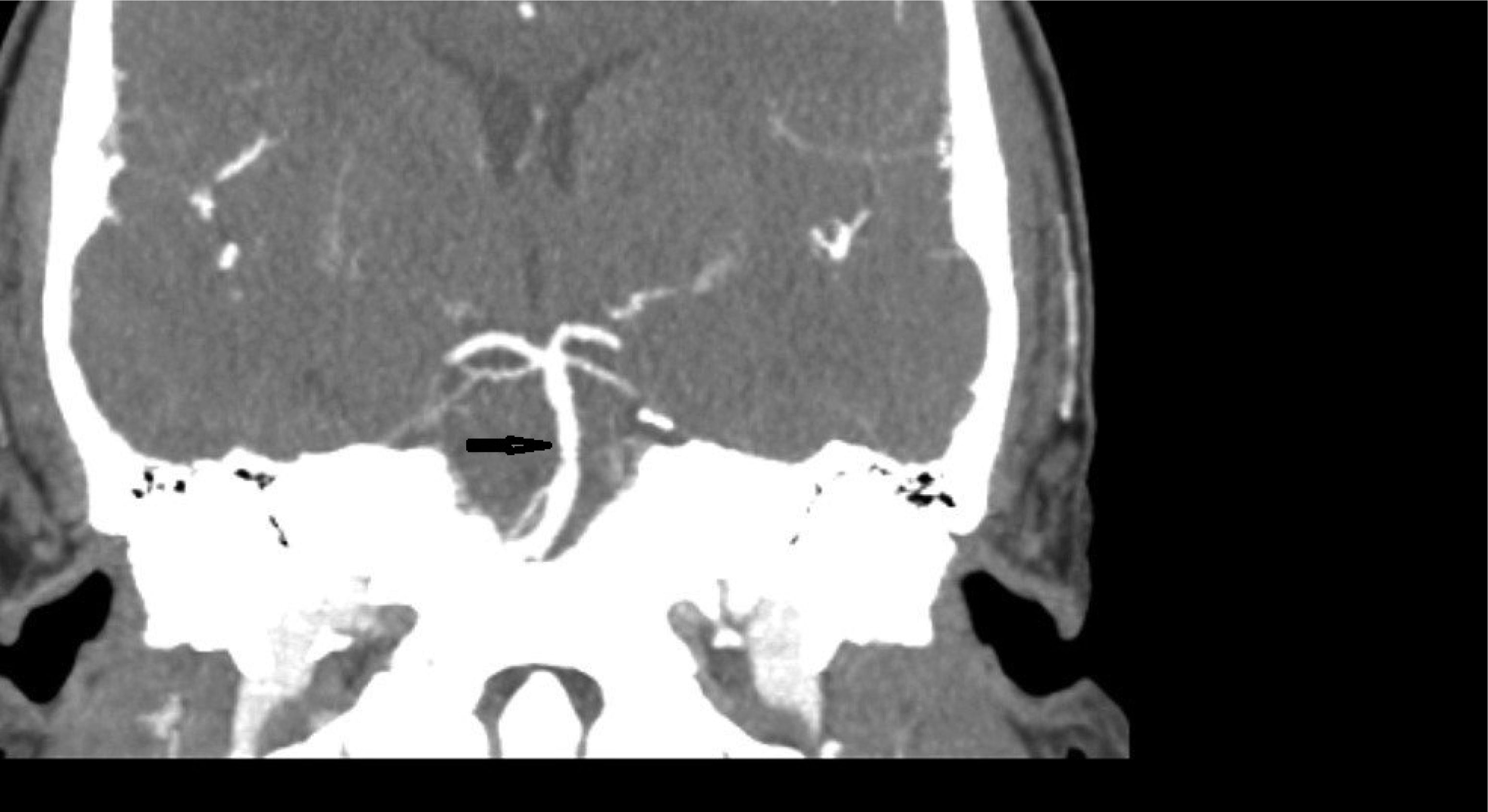
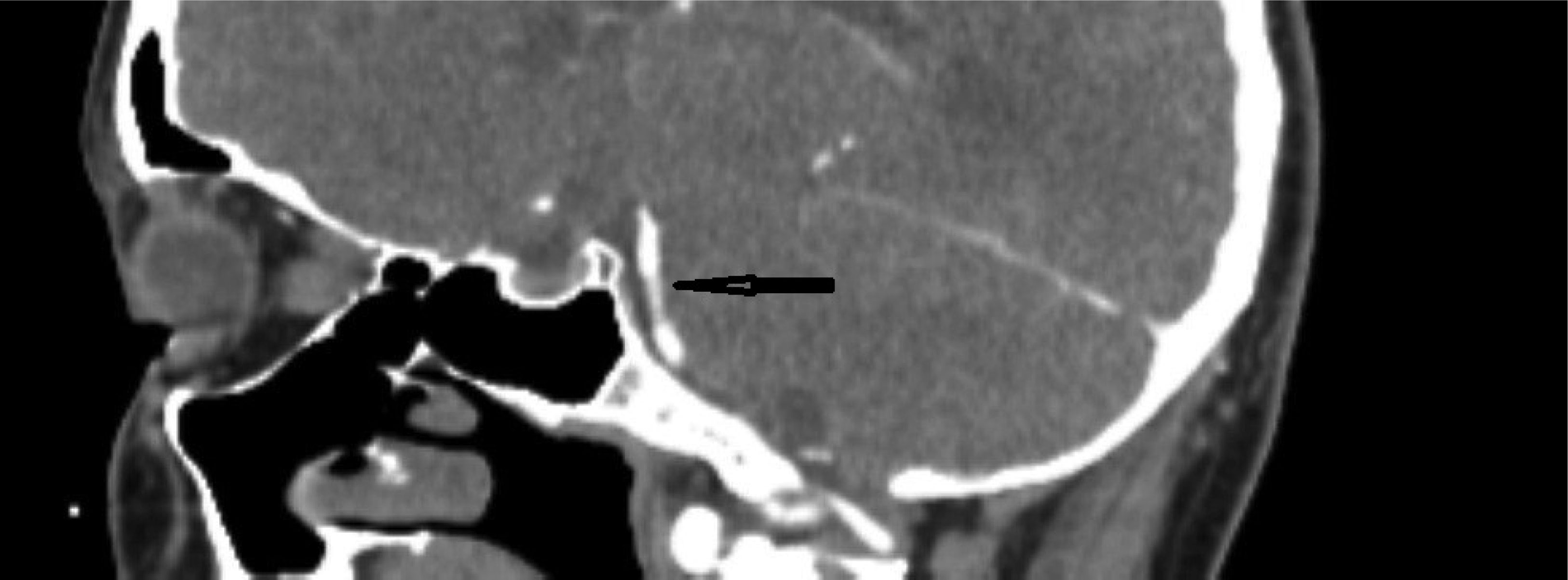
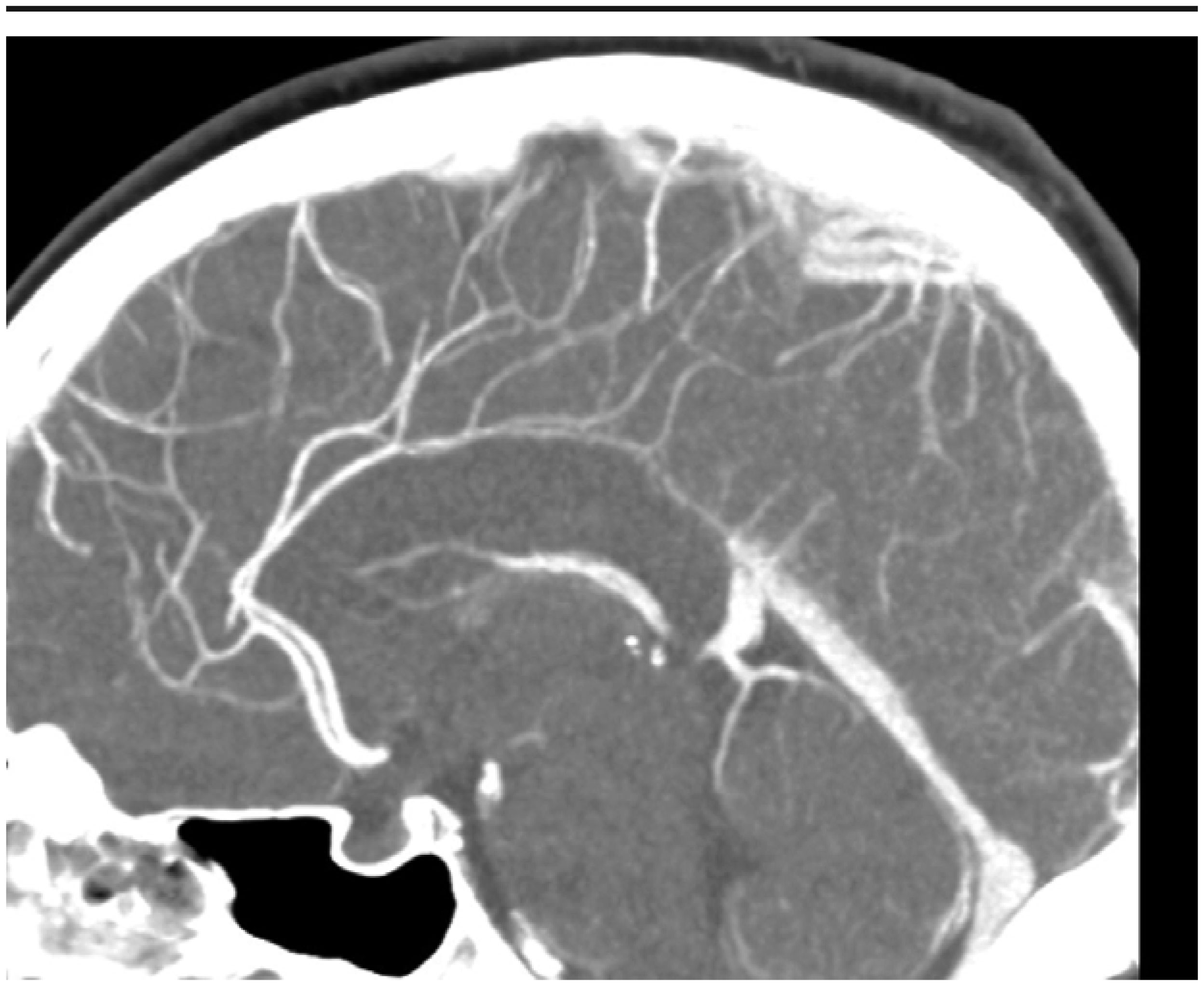
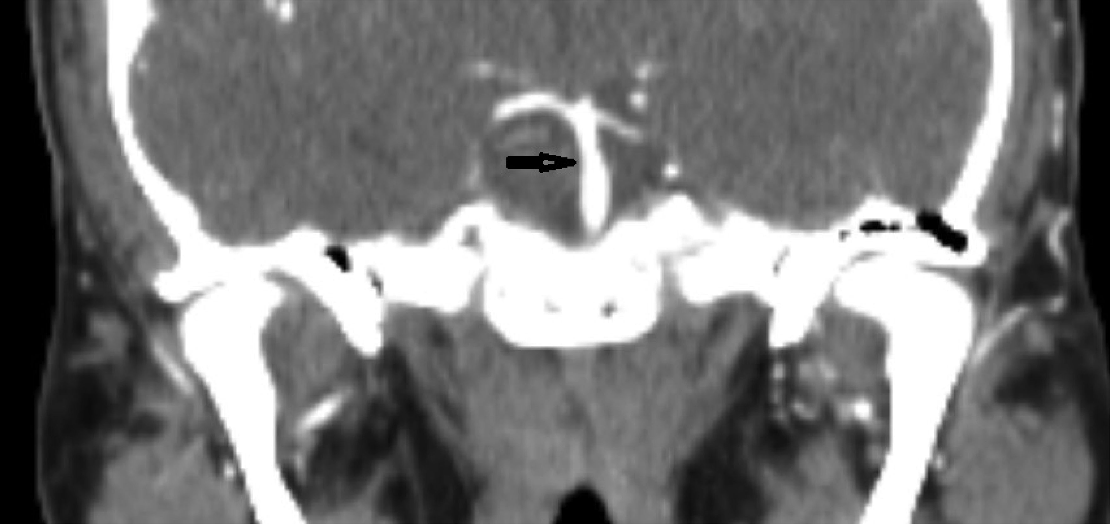
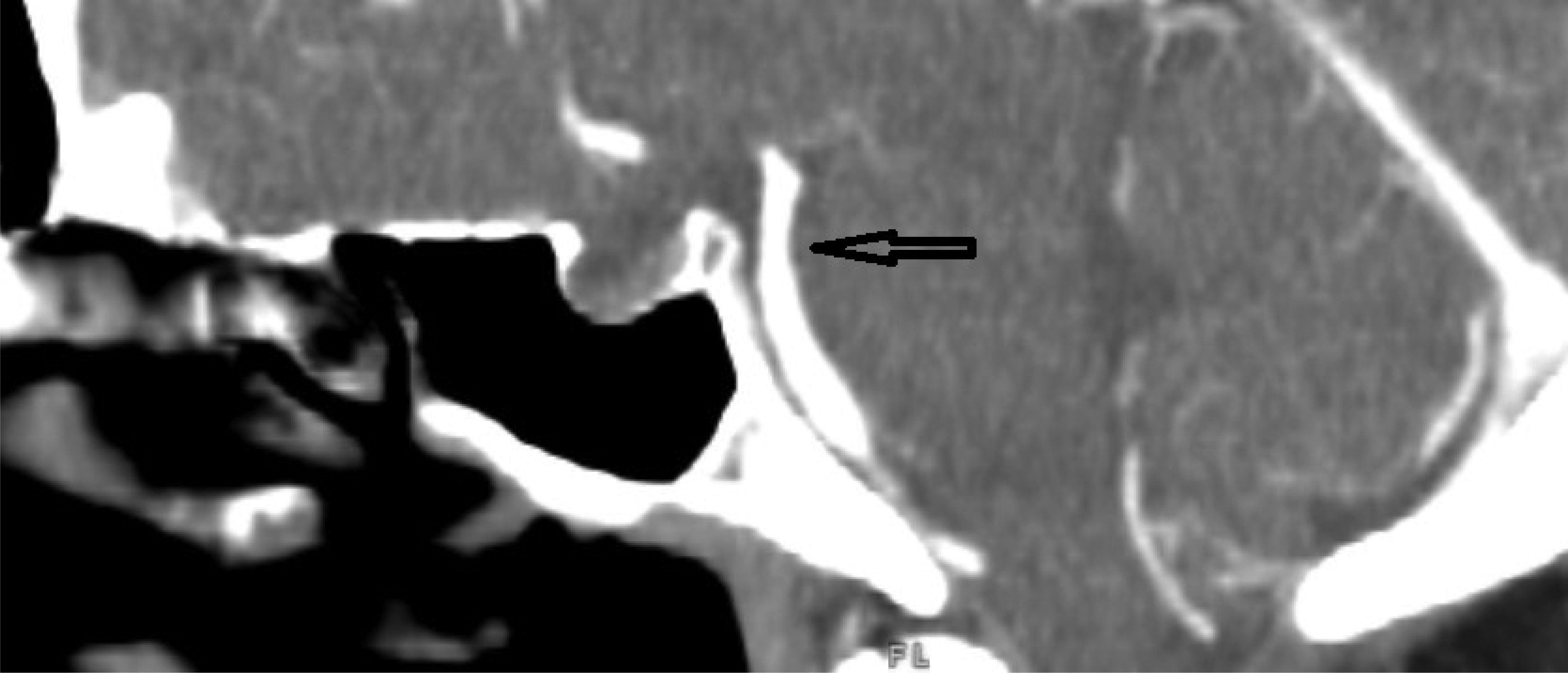
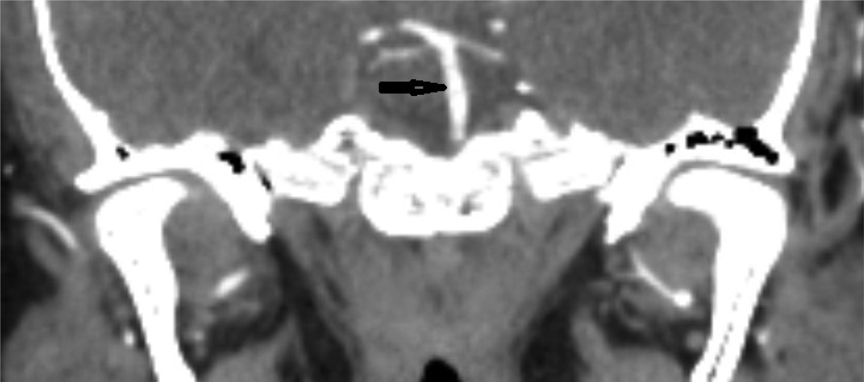
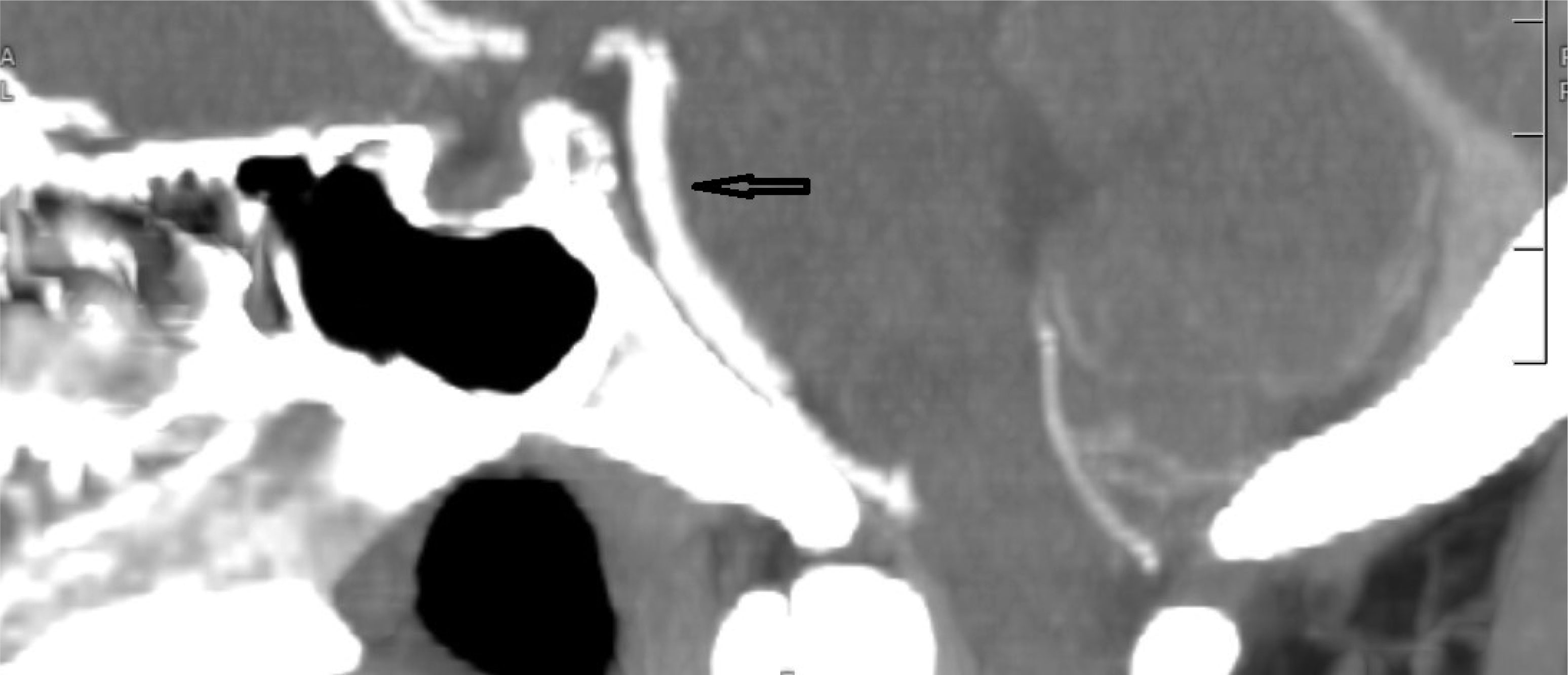
This case describes a 30-year-old Hispanic male who presented with a significant headache that started after a period of weightlifting and squatting. The patient was diagnosed with a basilar artery dissection. His only complaint was a headache that was exacerbated with exertion and sexual activity; there were no neurologic deficits. The diagnosis of basilar artery dissection was established and supported by findings on the CT angiogram of his head and neck. Basilar artery dissections are rarely seen, as they are likely underrecognized due to their varying clinical presentations; however, it is important to consider these phenomena due to the risk of progression and high morbidity rates.
Citation: Sahibjot Bhatia, Nimrit Gahoonia, Jeffrey Stenger, Forshing Lui. A rare case of basilar artery dissection[J]. AIMS Neuroscience, 2023, 10(2): 109-117. doi: 10.3934/Neuroscience.2023008
This case describes a 30-year-old Hispanic male who presented with a significant headache that started after a period of weightlifting and squatting. The patient was diagnosed with a basilar artery dissection. His only complaint was a headache that was exacerbated with exertion and sexual activity; there were no neurologic deficits. The diagnosis of basilar artery dissection was established and supported by findings on the CT angiogram of his head and neck. Basilar artery dissections are rarely seen, as they are likely underrecognized due to their varying clinical presentations; however, it is important to consider these phenomena due to the risk of progression and high morbidity rates.

| [1] |
Ruecker M, Furtner M, Knoflach M, et al. (2010) Basilar artery dissection: series of 12 consecutive cases and review of the literature. Cerebrovasc Dis 30: 267-276. https://doi.org/10.1159/000319069 
|
| [2] |
Yoshimoto Y, Hoya K, Tanaka Y, et al. (2005) Basilar artery dissection. J Neurosurg 102: 476-481. https://doi.org/10.3171/jns.2005.102.3.0476
|
| [3] |
Thanvi B, Munshi SK, Dawson SL, et al. (2005) Carotid and vertebral artery dissection syndromes. Postgrad Med J 81: 383-388. https://doi.org/10.1136/pgmj.2003.016774
|
| [4] | Yilmaza F, Arslana E, Ozlema M, et al. (2013) A Rare Presentation of Stroke: Basilary Artery Dissection. Journal of Medical Cases 4. https://doi.org/10.4021/jmc898w |
| [5] |
Wu Y, Chen H, Xing S, et al. (2020) Predisposing factors and radiological features in patients with internal carotid artery dissection or vertebral artery dissection. BMC Neurol 20: 445. https://doi.org/10.1186/s12883-020-02020-8
|
| [6] | Han Z, Leung T, Lam W, et al. (2007) Spontaneous basilar artery dissection. Hong Kong Med J . |
| [7] | Guinn KJ, Kurkchijski RG, Shen CA (2021) Vertebral artery dissection and high-intensity workouts. Proc (Bayl Univ Med Cent) 34: 708-709. https://doi.org/10.1080/08998280.2021.1935139 |
| [8] |
Kang K, Kim JH, Kim BK (2022) Exercise Headache Associated With an Arteriovenous Fistula of the External Carotid Artery. J Clin Neurol 18: 93-95. https://doi.org/10.3988/jcn.2022.18.1.93
|
| [9] | Scislicki P, Sztuba K, Klimkowicz-Mrowiec A, et al. (2021) Headache Associated with Sexual Activity-A Narrative Review of Literature. Medicina (Kaunas) 57. https://doi.org/10.3390/medicina57080735 |
| [10] |
Delasobera BE, Osborn SR, Davis JE (2012) Thunderclap headache with orgasm: a case of basilar artery dissection associated with sexual intercourse. J Emerg Med 43: e43-47. https://doi.org/10.1016/j.jemermed.2009.08.012
|
| [11] |
Mehdi E, Aralasmak A, Toprak H, et al. (2018) Craniocervical Dissections: Radiologic Findings, Pitfalls, Mimicking Diseases: A Pictorial Review. Curr Med Imaging Rev 14: 207-222. https://doi.org/10.2174/1573405613666170403102235
|
| [12] |
Kim BM, Suh SH, Park SI, et al. (2008) Management and clinical outcome of acute basilar artery dissection. AJNR Am J Neuroradiol 29: 1937-1941. https://doi.org/10.3174/ajnr.A1243
|
| [13] |
Debette S, Mazighi M, Bijlenga P, et al. (2021) ESO guideline for the management of extracranial and intracranial artery dissection. Eur Stroke J 6: XXXIX-LXXXVIII. https://doi.org/10.1177/23969873211046475
|
| [14] |
Daou B, Hammer C, Mouchtouris N, et al. (2017) Anticoagulation vs Antiplatelet Treatment in Patients with Carotid and Vertebral Artery Dissection: A Study of 370 Patients and Literature Review. Neurosurgery 80: 368-379. https://doi.org/10.1093/neuros/nyw086
|
Figures(7)

Sahibjot Bhatia, Nimrit Gahoonia, Jeffrey Stenger, Forshing Lui. A rare case of basilar artery dissection[J]. AIMS Neuroscience, 2023, 10(2): 109-117. doi: 10.3934/Neuroscience.2023008


 DownLoad: