Academic interest in understanding the role of financial technology (FinTech) in sustainable development has grown exponentially in recent years. Many studies have highlighted the context, yet no reviews have explored the integration of FinTech and sustainability through the lens of the banking aspect. Therefore, this study sheds light on the literature trends associated with FinTech and sustainable banking using an integrated bibliometric and systematic literature review (SLR). The bibliometric analysis explored publication trends, keyword analysis, top publisher, and author analysis. With the SLR approach, we pondered the theory-context-characteristics-methods (TCCM) framework with 44 articles published from 2002 to 2023. The findings presented a substantial nexus between FinTech and sustainable banking, showing an incremental interest among global scholars. We also provided a comprehensive finding regarding the dominant theories (i.e., technology acceptance model and autoregressive distributed lag model), specific contexts (i.e., industries and countries), characteristics (i.e., independent, dependent, moderating, and mediating variables), and methods (i.e., research approaches and tools). This review is the first to identify the less explored tie between FinTech and sustainable banking. The findings may help policymakers, banking service providers, and academicians understand the necessity of FinTech in sustainable banking. The future research agenda of this review will also facilitate future researchers to explore the research domain to find new insights.
Citation: Md. Shahinur Rahman, Iqbal Hossain Moral, Md. Abdul Kaium, Gertrude Arpa Sarker, Israt Zahan, Gazi Md. Shakhawat Hossain, Md Abdul Mannan Khan. FinTech in sustainable banking: An integrated systematic literature review and future research agenda with a TCCM framework[J]. Green Finance, 2024, 6(1): 92-116. doi: 10.3934/GF.2024005
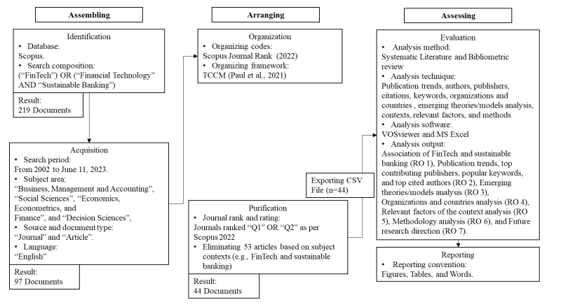
Academic interest in understanding the role of financial technology (FinTech) in sustainable development has grown exponentially in recent years. Many studies have highlighted the context, yet no reviews have explored the integration of FinTech and sustainability through the lens of the banking aspect. Therefore, this study sheds light on the literature trends associated with FinTech and sustainable banking using an integrated bibliometric and systematic literature review (SLR). The bibliometric analysis explored publication trends, keyword analysis, top publisher, and author analysis. With the SLR approach, we pondered the theory-context-characteristics-methods (TCCM) framework with 44 articles published from 2002 to 2023. The findings presented a substantial nexus between FinTech and sustainable banking, showing an incremental interest among global scholars. We also provided a comprehensive finding regarding the dominant theories (i.e., technology acceptance model and autoregressive distributed lag model), specific contexts (i.e., industries and countries), characteristics (i.e., independent, dependent, moderating, and mediating variables), and methods (i.e., research approaches and tools). This review is the first to identify the less explored tie between FinTech and sustainable banking. The findings may help policymakers, banking service providers, and academicians understand the necessity of FinTech in sustainable banking. The future research agenda of this review will also facilitate future researchers to explore the research domain to find new insights.

| [1] |
Abdul-Rahim R, Bohari SA, Aman A, et al. (2022) Benefit–risk perceptions of FinTech adoption for sustainability from bank consumers' perspective: The moderating role of fear of COVID-19. Sustainability 14: 8357. https://doi.org/10.3390/su14148357 doi: 10.3390/su14148357

|
| [2] |
Aduba JJ (2021) On the determinants, gains and challenges of electronic banking adoption in Nigeria. Int J Soc Econ 48: 1021–1043. https://doi.org/10.1108/IJSE-07-2020-0452 doi: 10.1108/IJSE-07-2020-0452
|
| [3] |
Alaabed A, Masih M, Mirakhor A (2016) Investigating risk shifting in Islamic banks in the dual banking systems of OIC member countries: an application of two-step dynamic GMM. Risk Manage 18: 236–263. https://doi.org/10.1057/s41283-016-0007-3 doi: 10.1057/s41283-016-0007-3
|
| [4] |
Aracil E, Nájera-Sánchez JJ, Forcadell FJ (2021) Sustainable banking: A literature review and integrative framework. Financ Res Lett 42: 101932. https://doi.org/10.1016/j.frl.2021.101932 doi: 10.1016/j.frl.2021.101932
|
| [5] | Ashrafi DM, Dovash RH, Kabir MR (2022) Determinants of fintech service continuance behavior: moderating role of transaction security and trust. J Global Bus Technol 18. Available from: https://www.proquest.com/docview/2766511260?pq-origsite = gscholar & fromopenview = true & sourcetype = Scholarly%20Journals. |
| [6] |
Ashta A, Herrmann H (2021) Artificial intelligence and fintech: An overview of opportunities and risks for banking, investments, and microfinance. Strateg Change 30: 211–222. https://doi.org/10.1002/jsc.2404 doi: 10.1002/jsc.2404
|
| [7] |
Banna H, Hassan MK, Ahmad R, et al. (2022) Islamic banking stability amidst the COVID-19 pandemic: the role of digital financial inclusion. Int J Islamic Middle 15: 310–330. https://doi.org/10.1108/IMEFM-08-2020-0389 doi: 10.1108/IMEFM-08-2020-0389
|
| [8] |
Boratyńska K (2019) Impact of digital transformation on value creation in Fintech services: an innovative approach. J Promot Manage 25: 631–639. https://doi.org/10.1080/10496491.2019.1585543 doi: 10.1080/10496491.2019.1585543
|
| [9] |
Bose S, Khan HZ, Rashid A, et al. (2018) What drives green banking disclosure? An institutional and corporate governance perspective. Asia Pac J Manage 35: 501–527. https://doi.org/10.1007/s10490-017-9528-x doi: 10.1007/s10490-017-9528-x
|
| [10] |
Brahmi M, Esposito L, Parziale A, et al. (2023) The role of greener innovations in promoting financial inclusion to achieve carbon neutrality: an integrative review. Economies 11: 194. https://doi.org/10.3390/economies11070194 doi: 10.3390/economies11070194
|
| [11] |
Çera G, Phan QPT, Androniceanu A, et al. (2020) Financial capability and technology implications for online shopping. EaM Ekon Manag. https://doi.org/10.15240/tul/001/2020-2-011 doi: 10.15240/tul/001/2020-2-011
|
| [12] |
Chang HY, Liang LW, Liu YL (2021) Using environmental, social, governance (ESG) and financial indicators to measure bank cost efficiency in Asia. Sustainability 13: 11139. https://doi.org/10.3390/su132011139 doi: 10.3390/su132011139
|
| [13] |
Coffie CPK, Zhao H, Adjei Mensah I (2020) Panel econometric analysis on mobile payment transactions and traditional banks effort toward financial accessibility in Sub-Sahara Africa. Sustainability 12: 895. https://doi.org/10.3390/su12030895 doi: 10.3390/su12030895
|
| [14] |
Cumming D, Johan S, Reardon R (2023) Global fintech trends and their impact on international business: a review. Multinatl Bus Rev 31: 413–436. https://doi.org/10.1108/MBR-05-2023-0077 doi: 10.1108/MBR-05-2023-0077
|
| [15] |
Danladi S, Prasad M, Modibbo UM, et al. (2023) Attaining Sustainable Development Goals through Financial Inclusion: Exploring Collaborative Approaches to Fintech Adoption in Developing Economies. Sustainability 15: 13039. https://doi.org/10.3390/su151713039 doi: 10.3390/su151713039
|
| [16] |
Davis FD, Bagozzi RP, Warshaw PR (1989) User acceptance of computer technology: A comparison of two theoretical models. Manage Sci 35: 982–1003. https://doi.org/10.1287/mnsc.35.8.982 doi: 10.1287/mnsc.35.8.982
|
| [17] |
Dewi IGAAO, Dewi IGAAP (2017) Corporate social responsibility, green banking, and going concern on banking company in Indonesia stock exchange. Int J Soc Sci Hum 1: 118–134. https://doi.org/10.29332/ijssh.v1n3.65 doi: 10.29332/ijssh.v1n3.65
|
| [18] |
Diep NTN, Canh TQ (2022) Impact analysis of peer-to-peer Fintech in Vietnam's banking industry. J Int Stud 15. https://doi.org/10.14254/2071-8330.2022/15-3/12 doi: 10.14254/2071-8330.2022/15-3/12
|
| [19] |
Dong Y, Chung M, Zhou C, et al. (2018) Banking on "mobile money": The implications of mobile money services on the value chain. Manuf Serv Oper Manag. https://doi.org/10.1287/msom.2018.0717 doi: 10.1287/msom.2018.0717
|
| [20] |
Eisingerich AB, Bell SJ (2008) Managing networks of interorganizational linkages and sustainable firm performance in business‐to‐business service contexts. J Serv Mark 22: 494–504. https://doi.org/10.1108/08876040810909631 doi: 10.1108/08876040810909631
|
| [21] |
Ellili NOD (2022) Is there any association between FinTech and sustainability? Evidence from bibliometric review and content analysis. J Financ Serv Mark 28: 748–762. https://doi.org/10.1057/s41264-022-00200-w doi: 10.1057/s41264-022-00200-w
|
| [22] |
Fenwick M, Vermeulen EP (2020) Banking and regulatory responses to FinTech revisited-building the sustainable financial service'ecosystems' of tomorrow. Singap J Legal Stud 2020: 165–189. https://doi.org/10.2139/ssrn.3446273 doi: 10.2139/ssrn.3446273
|
| [23] |
Gangi F, Meles A, Daniele LM, et al. (2021) Socially responsible investment (SRI): from niche to mainstream. The Evolution of Sustainable Investments and Finance: Theoretical Perspectives and New Challenges, 1–58. https://doi.org/10.1007/978-3-030-70350-9_1 doi: 10.1007/978-3-030-70350-9_1
|
| [24] |
Gbongli K, Xu Y, Amedjonekou KM, et al. (2020) Evaluation and classification of mobile financial services sustainability using structural equation modeling and multiple criteria decision-making methods. Sustainability 12: 1288. https://doi.org/10.3390/su12041288 doi: 10.3390/su12041288
|
| [25] |
Goodell JW, Kumar S, Lim WM, et al. (2021) Artificial intelligence and machine learning in finance: Identifying foundations, themes, and research clusters from bibliometric analysis. J Behav Exp Financ 32: 100577. https://doi.org/10.1016/j.jbef.2021.100577 doi: 10.1016/j.jbef.2021.100577
|
| [26] |
Gozman D, Willcocks L (2019) The emerging Cloud Dilemma: Balancing innovation with cross-border privacy and outsourcing regulations. J Bus Res 97: 235–256. https://doi.org/10.1016/j.jbusres.2018.06.006 doi: 10.1016/j.jbusres.2018.06.006
|
| [27] |
Gruin J, Knaack P (2020) Not just another shadow bank: Chinese authoritarian capitalism and the 'developmental'promise of digital financial innovation. New Polit Econ 25: 370–387. https://doi.org/10.1080/13563467.2018.1562437 doi: 10.1080/13563467.2018.1562437
|
| [28] |
Guang-Wen Z, Siddik AB (2023) The effect of Fintech adoption on green finance and environmental performance of banking institutions during the COVID-19 pandemic: the role of green innovation. Environ Sci Pollut Res 30: 25959–25971. https://doi.org/10.1007/s11356-022-23956-z doi: 10.1007/s11356-022-23956-z
|
| [29] |
Guo Y, Holland J, Kreander N (2014) An exploration of the value creation process in bank-corporate communications. J Commun manage 18: 254–270. https://doi.org/10.1108/JCOM-10-2012-0079 doi: 10.1108/JCOM-10-2012-0079
|
| [30] | Hassan MK, Rabbani MR, Ali MAM (2020) Challenges for the Islamic Finance and banking in post COVID era and the role of Fintech. J Econ Coop Dev 41: 93–116. Available from: https://www.proquest.com/docview/2503186452?pq-origsite = gscholar & fromopenview = true & sourcetype = Scholarly%20Journals. |
| [31] | Hassan SM, Rahman Z, Paul J (2022) Consumer ethics: A review and research agenda. Psychol Market 39: 111–130. |
| [32] |
He J, Zhang S (2022) How digitalized interactive platforms create new value for customers by integrating B2B and B2C models? An empirical study in China. J Bus Res 142: 694–706. https://doi.org/10.1016/j.jbusres.2022.01.004 doi: 10.1016/j.jbusres.2022.01.004
|
| [33] |
Hommel K, Bican PM (2020) Digital entrepreneurship in finance: Fintechs and funding decision criteria. Sustainability 12: 8035. https://doi.org/10.3390/su12198035 doi: 10.3390/su12198035
|
| [34] |
Hyun S (2022) Current Status and Challenges of Green Digital Finance in Korea. Green Digital Finance and Sustainable Development Goals, 243–261. https://doi.org/10.1007/978-981-19-2662-4_12 doi: 10.1007/978-981-19-2662-4_12
|
| [35] |
Ⅱ WWC, Demrig I (2002) Investment and capitalisation of firms in the USA. Int J Technol Manage 24: 391–418. https://doi.org/10.1504/IJTM.2002.003062 doi: 10.1504/IJTM.2002.003062
|
| [36] |
Iman N (2018) Is mobile payment still relevant in the fintech era? Electron Commer Res Appl 30: 72–82. https://doi.org/10.1016/j.elerap.2018.05.009 doi: 10.1016/j.elerap.2018.05.009
|
| [37] |
Ji F, Tia A (2022) The effect of blockchain on business intelligence efficiency of banks. Kybernetes 51: 2652–2668. https://doi.org/10.1108/K-10-2020-0668 doi: 10.1108/K-10-2020-0668
|
| [38] |
Jibril AB, Kwarteng MA, Botchway RK, et al. (2020) The impact of online identity theft on customers' willingness to engage in e-banking transaction in Ghana: A technology threat avoidance theory. Cogent Bus Manag 7: 1832825. https://doi.org/10.1080/23311975.2020.1832825 doi: 10.1080/23311975.2020.1832825
|
| [39] |
Khan A, Goodell JW, Hassan MK, et al. (2022) A bibliometric review of finance bibliometric papers. Financ Res Lett 47: 102520. https://doi.org/10.1016/j.frl.2021.102520 doi: 10.1016/j.frl.2021.102520
|
| [40] |
Khan HU, Sohail M, Nazir S, et al. (2023) Role of authentication factors in Fin-tech mobile transaction security. J Big Data 10: 138. https://doi.org/10.1186/s40537-023-00807-3 doi: 10.1186/s40537-023-00807-3
|
| [41] |
Kumar S, Lim WM, Sivarajah U, et al. (2023) Artificial intelligence and blockchain integration in business: trends from a bibliometric-content analysis. Inform Syst Front 25: 871–896. https://doi.org/10.1007/s10796-022-10279-0 doi: 10.1007/s10796-022-10279-0
|
| [42] |
Kumari A, Devi NC (2022) The Impact of FinTech and Blockchain Technologies on Banking and Financial Services. Technol Innov Manage Rev 12. https://doi.org/10.22215/timreview/1481 doi: 10.22215/timreview/1481
|
| [43] |
Lai X, Yue S, Guo C, et al. (2023) Does FinTech reduce corporate excess leverage? Evidence from China. Econ Anal Policy 77: 281–299. https://doi.org/10.1016/j.eap.2022.11.017 doi: 10.1016/j.eap.2022.11.017
|
| [44] |
Lee WS, Sohn SY (2017) Identifying emerging trends of financial business method patents. Sustainability 9: 1670. https://doi.org/10.3390/su9091670 doi: 10.3390/su9091670
|
| [45] |
Lekakos G, Vlachos P, Koritos C (2014) Green is good but is usability better? Consumer reactions to environmental initiatives in e-banking services. Ethics Inf Technol 16: 103–117. https://doi.org/10.1007/s10676-014-9337-6 doi: 10.1007/s10676-014-9337-6
|
| [46] | Mądra-Sawicka M (2020) Financial management in the big data era. In Management in the Era of Big Data, 71–81, Auerbach Publications. https://doi.org/10.1201/9781003057291-6 |
| [47] |
Mejia-Escobar JC, González-Ruiz JD, Duque-Grisales E (2020) Sustainable financial products in the Latin America banking industry: Current status and insights. Sustainability 12: 5648. https://doi.org/10.3390/su12145648 doi: 10.3390/su12145648
|
| [48] | Mhlanga D (2023) FinTech for Sustainable Development in Emerging Markets with Case Studies. In FinTech and Artificial Intelligence for Sustainable Development: The Role of Smart Technologies in Achieving Development Goals, 337–363, Springer. https://doi.org/10.1007/978-3-031-37776-1_15 |
| [49] |
Mohr I, Fuxman L, Mahmoud AB (2022) A triple-trickle theory for sustainable fashion adoption: the rise of a luxury trend. J Fash Mark Manag Int J 26: 640–660. https://doi.org/10.1108/JFMM-03-2021-0060 doi: 10.1108/JFMM-03-2021-0060
|
| [50] |
Muniz Jr AM, Schau HJ (2005) Religiosity in the abandoned Apple Newton brand community. J Consum Res 31: 737–747. https://doi.org/10.1086/426607 doi: 10.1086/426607
|
| [51] |
Naruetharadhol P, Ketkaew C, Hongkanchanapong N, et al. (2021) Factors affecting sustainable intention to use mobile banking services. Sage Open 11: 21582440211029925. https://doi.org/10.1177/21582440211029925 doi: 10.1177/21582440211029925
|
| [52] |
Nenavath S (2022) Impact of fintech and green finance on environmental quality protection in India: By applying the semi-parametric difference-in-differences (SDID). Renew Energ 193: 913–919. https://doi.org/10.1016/j.renene.2022.05.020 doi: 10.1016/j.renene.2022.05.020
|
| [53] |
Nosratabadi S, Pinter G, Mosavi A, et al. (2020) Sustainable banking; evaluation of the European business models. Sustainability 12: 2314. https://doi.org/10.3390/su12062314 doi: 10.3390/su12062314
|
| [54] |
Ortas E, Burritt RL, Moneva JM (2013) Socially Responsible Investment and cleaner production in the Asia Pacific: does it pay to be good? J Cleaner Prod 52: 272–280. https://doi.org/10.1016/j.jclepro.2013.02.024 doi: 10.1016/j.jclepro.2013.02.024
|
| [55] |
Oseni UA, Adewale AA, Omoola SO (2018) The feasibility of online dispute resolution in the Islamic banking industry in Malaysia: An empirical legal analysis. Int J Law Manag 60: 34–54. https://doi.org/10.1108/IJLMA-06-2016-0057 doi: 10.1108/IJLMA-06-2016-0057
|
| [56] |
Paiva BM, Ferreira FA, Carayannis EG, et al. (2021) Strategizing sustainability in the banking industry using fuzzy cognitive maps and system dynamics. Int J Sustain Dev World Ecol 28: 93–108. https://doi.org/10.1080/13504509.2020.1782284 doi: 10.1080/13504509.2020.1782284
|
| [57] |
Parmentola A, Petrillo A, Tutore I, et al. (2022) Is blockchain able to enhance environmental sustainability? A systematic review and research agenda from the perspective of Sustainable Development Goals (SDGs). Bus Strateg Environ 31: 194–217. https://doi.org/10.1002/bse.2882 doi: 10.1002/bse.2882
|
| [58] |
Paul J, Lim WM, O'Cass A, et al. (2021) Scientific procedures and rationales for systematic literature reviews (SPAR‐4‐SLR). Int J Consum Stud 45: O1–O16. https://doi.org/10.1111/ijcs.12695 doi: 10.1111/ijcs.12695
|
| [59] |
Puschmann T, Hoffmann CH, Khmarskyi V (2020) How green FinTech can alleviate the impact of climate change—the case of Switzerland. Sustainability 12: 10691. https://doi.org/10.3390/su122410691 doi: 10.3390/su122410691
|
| [60] |
Rahman S, Moral IH, Hassan M, et al. (2022) A systematic review of green finance in the banking industry: perspectives from a developing country. Green Financ 4: 347–363. https://doi.org/10.3934/GF.2022017 doi: 10.3934/GF.2022017
|
| [61] |
Ryu HS, Ko KS (2020) Sustainable development of Fintech: Focused on uncertainty and perceived quality issues. Sustainability 12: 7669. https://doi.org/10.3390/su12187669 doi: 10.3390/su12187669
|
| [62] |
Sagnier C, Loup-Escande E, Lourdeaux D, et al. (2020) User acceptance of virtual reality: an extended technology acceptance model. Int J Hum–Comput Interact 36: 993–1007. https://doi.org/10.1080/10447318.2019.1708612 doi: 10.1080/10447318.2019.1708612
|
| [63] |
Sethi P, Chakrabarti D, Bhattacharjee S (2020) Globalization, financial development and economic growth: Perils on the environmental sustainability of an emerging economy. J Policy Model 42: 520–535. https://doi.org/10.1016/j.jpolmod.2020.01.007 doi: 10.1016/j.jpolmod.2020.01.007
|
| [64] |
Singh RK, Mishra R, Gupta S, et al. (2023) Blockchain applications for secured and resilient supply chains: A systematic literature review and future research agenda. Comput Ind Eng 175: 108854. https://doi.org/10.1016/j.cie.2022.108854 doi: 10.1016/j.cie.2022.108854
|
| [65] |
Sun Y, Luo B, Wang S, et al. (2021) What you see is meaningful: Does green advertising change the intentions of consumers to purchase eco‐labeled products? Bus Strateg Environ 30: 694–704. https://doi.org/10.1002/bse.2648 doi: 10.1002/bse.2648
|
| [66] |
Talom FSG, Tengeh RK (2019) The impact of mobile money on the financial performance of the SMEs in Douala, Cameroon. Sustainability 12: 183. https://doi.org/10.3390/su12010183 doi: 10.3390/su12010183
|
| [67] |
Taneja S, Siraj A, Ali L, et al. (2023) Is fintech implementation a strategic step for sustainability in today's changing landscape? An empirical investigation. IEEE T Eng Manage. https://doi.org/10.3390/su12010183 doi: 10.3390/su12010183
|
| [68] |
Tara K, Singh S, Kumar R, et al. (2019) Geographical locations of banks as an influencer for green banking adoption. Prabandhan: Indian J Manag 12: 21–35. https://doi.org/10.17010/pijom/2019/v12i1/141425 doi: 10.17010/pijom/2019/v12i1/141425
|
| [69] |
Tchamyou VS, Erreygers G, Cassimon D (2019) Inequality, ICT and financial access in Africa. Technol Forecast Soc Change 139: 169–184. https://doi.org/10.1016/j.techfore.2018.11.004 doi: 10.1016/j.techfore.2018.11.004
|
| [70] |
Tripathi R (2023) Framework of green finance to attain sustainable development goals: an empirical evidence from the TCCM approach. Benchmarking. https://doi.org/10.1108/BIJ-05-2023-0311 doi: 10.1108/BIJ-05-2023-0311
|
| [71] |
Truby J, Brown R, Dahdal A (2020) Banking on AI: mandating a proactive approach to AI regulation in the financial sector. Law Financ Mark Rev 14: 110–120. https://doi.org/10.1080/17521440.2020.1760454 doi: 10.1080/17521440.2020.1760454
|
| [72] |
Tsindeliani IA, Proshunin MM, Sadovskaya TD, et al. (2022) Digital transformation of the banking system in the context of sustainable development. J Money Laund Contro 25: 165–180. https://doi.org/10.1108/JMLC-02-2021-0011 doi: 10.1108/JMLC-02-2021-0011
|
| [73] |
Ullah A, Pinglu C, Ullah S, et al. (2023) Impact of intellectual capital efficiency on financial stability in banks: Insights from an emerging economy. Int J Financ Econ 28: 1858–1871. https://doi.org/10.1002/ijfe.2512 doi: 10.1002/ijfe.2512
|
| [74] |
Yadav MS (2010) The decline of conceptual articles and implications for knowledge development. J Mark 74: 1–19. https://doi.org/10.1509/jmkg.74.1.1 doi: 10.1509/jmkg.74.1.1
|
| [75] |
Yan C, Siddik AB, Yong L, et al. (2022) A two-staged SEM-artificial neural network approach to analyze the impact of FinTech adoption on the sustainability performance of banking firms: The mediating effect of green finance and innovation. Systems 10: 148. https://doi.org/10.3390/systems10050148 doi: 10.3390/systems10050148
|
| [76] |
Yang C, Masron TA (2022) Impact of digital finance on energy efficiency in the context of green sustainable development. Sustainability 14: 11250. https://doi.org/10.3390/su14181125 doi: 10.3390/su14181125
|
| [77] |
Yigitcanlar T, Cugurullo F (2020) The sustainability of artificial intelligence: An urbanistic viewpoint from the lens of smart and sustainable cities. Sustainability 12: 8548. https://doi.org/10.3390/su1220854 doi: 10.3390/su1220854
|
| [78] |
Zhang Y (2023) Impact of green finance and environmental protection on green economic recovery in South Asian economies: mediating role of FinTech. Econ Chang Restruct 56: 2069–2086. https://doi.org/10.1007/s10644-023-09500-0 doi: 10.1007/s10644-023-09500-0
|
| [79] | Zhao D, Strotmann A (2015) Analysis and visualization of citation networks. Morgan & Claypool Publishers. |
| [80] |
Zhao Q, Tsai PH, Wang JL (2019) Improving financial service innovation strategies for enhancing china's banking industry competitive advantage during the fintech revolution: A Hybrid MCDM model. Sustainability 11: 1419. https://doi.org/10.3390/su11051419 doi: 10.3390/su11051419
|
| [81] |
Zuo L, Strauss J, Zuo L (2021) The digitalization transformation of commercial banks and its impact on sustainable efficiency improvements through investment in science and technology. Sustainability 13: 11028. https://doi.org/10.3390/su131911028 doi: 10.3390/su131911028
|


Figures(6) / Tables(7)

Md. Shahinur Rahman, Iqbal Hossain Moral, Md. Abdul Kaium, Gertrude Arpa Sarker, Israt Zahan, Gazi Md. Shakhawat Hossain, Md Abdul Mannan Khan. FinTech in sustainable banking: An integrated systematic literature review and future research agenda with a TCCM framework[J]. Green Finance, 2024, 6(1): 92-116. doi: 10.3934/GF.2024005


 DownLoad: