


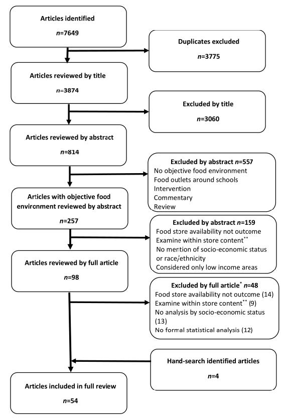
Citation: Karen E. Lamb, Lukar E. Thornton, Ester Cerin, Kylie Ball. Statistical Approaches Used to Assess the Equity of Access to Food Outlets: A Systematic Review[J]. AIMS Public Health, 2015, 2(3): 358-401. doi: 10.3934/publichealth.2015.3.358
| [1] | Yassine Charabi, Sabah Abdul-Wahab . The optimal sizing and performance assessment of a hybrid renewable energy system for a mini-gird in an exclave territory. AIMS Energy, 2020, 8(4): 669-685. doi: 10.3934/energy.2020.4.669 |
| [2] | S. Vinoth John Prakash, P.K. Dhal . Cost optimization and optimal sizing of standalone biomass/diesel generator/wind turbine/solar microgrid system. AIMS Energy, 2022, 10(4): 665-694. doi: 10.3934/energy.2022032 |
| [3] | Abshir Ashour, Taib Iskandar Mohamad, Kamaruzzaman Sopian, Norasikin Ahmad Ludin, Khaled Alzahrani, Adnan Ibrahim . Performance optimization of a photovoltaic-diesel hybrid power system for Yanbu, Saudi Arabia. AIMS Energy, 2021, 9(6): 1260-1273. doi: 10.3934/energy.2021058 |
| [4] | Tilahun Nigussie, Wondwossen Bogale, Feyisa Bekele, Edessa Dribssa . Feasibility study for power generation using off- grid energy system from micro hydro-PV-diesel generator-battery for rural area of Ethiopia: The case of Melkey Hera village, Western Ethiopia. AIMS Energy, 2017, 5(4): 667-690. doi: 10.3934/energy.2017.4.667 |
| [5] | Sulabh Sachan . Integration of electric vehicles with optimum sized storage for grid connected photo-voltaic system. AIMS Energy, 2017, 5(6): 997-1012. doi: 10.3934/energy.2017.6.997 |
| [6] | Z. Ismaila, O. A. Falode, C. J. Diji, R. A. Kazeem, O. M. Ikumapayi, M. O. Petinrin, A. A. Awonusi, S. O. Adejuwon, T-C. Jen, S. A. Akinlabi, E. T. Akinlabi . Evaluation of a hybrid solar power system as a potential replacement for urban residential and medical economic activity areas in southern Nigeria. AIMS Energy, 2023, 11(2): 319-336. doi: 10.3934/energy.2023017 |
| [7] | Md. Mehadi Hasan Shamim, Sidratul Montaha Silmee, Md. Mamun Sikder . Optimization and cost-benefit analysis of a grid-connected solar photovoltaic system. AIMS Energy, 2022, 10(3): 434-457. doi: 10.3934/energy.2022022 |
| [8] | K. M. S. Y. Konara, M. L. Kolhe, Arvind Sharma . Power dispatching techniques as a finite state machine for a standalone photovoltaic system with a hybrid energy storage. AIMS Energy, 2020, 8(2): 214-230. doi: 10.3934/energy.2020.2.214 |
| [9] | Syed Sabir Hussain Rizvi, Krishna Teerth Chaturvedi, Mohan Lal Kolhe . A review on peak shaving techniques for smart grids. AIMS Energy, 2023, 11(4): 723-752. doi: 10.3934/energy.2023036 |
| [10] | Manali Raman, P. Meena, V. Champa, V. Prema, Priya Ranjan Mishra . Techno-economic assessment of microgrid in rural India considering incremental load growth over years. AIMS Energy, 2022, 10(4): 900-921. doi: 10.3934/energy.2022041 |
Diesel generator sets, which are comprised of an internal combustion engine and coupled electric generator and controller, are commonly used in microgrid applications for backup power and off-grid power in remote locations where utility interconnections are not possible. Hybrid microgrids, which add additional DC energy sources via AC coupling to the AC generator through power electronic converters, offer an attractive alternative. Examples of DC sources include fuel cells, photovoltaic (PV) cells, and wind turbines. This hybrid approach has been shown to be economical in many off-grid applications [1,2,3,4,5,6]. Reducing fuel requirements and providing an alternative to installing uneconomical distribution feeders to remote locations are key components to the economic viability of off-grid hybrid microgrids in comparison to grid-tied system. When grid-tied, hybrid sources of energy can use the grid interface to help balance demand and generation while off-grid hybrid system often require energy storage through batteries or rapid load shedding to maintain system stability.
Energy storage, for example battery banks, can be coupled into the hybrid system through a power electronic converter. Energy storage through batteries provides much flexibility in operation of hybrid microgrids but typically exhibit short lifespan (< 10 years) and must be properly controlled to ensure system operation as detailed in [7]. More specifically, state of charge, depth/rate of discharge, and operational temperature are important factors that dictate the reliability and viability of battery storage systems in microgrids. Studies have shown that “within 6-24 months, 50-70% of solar PV home systems are not working as expected” [8]. The main failure mode in these systems lies within the battery storage system and is the result of improper system design, operation, or maintenance. As a result, it would be advantageous to reduce or eliminate the need of energy storage in hybrid microgrids. Demand response (DR) is an alternative that can help reduce the need of energy storage.
The concept of DR is to alter the electric usage by user in response to system operation. In grid-tied applications this is often desirable due to economic incentives [9,10,11] and research has shown that coupling DR with PV energy sources can be economically viable in such applications [12,13]. In off-grid applications DR could be a viable alternative, or complimentary technology, to reduce the use of battery storage. More specifically, “mismatch between supply and demand in microgri ds can be overcome by effectively utilizing distributed energy resources and/or encouraging demand side management” [14]. Some recent work has been developing DR techniques designed to be coupled with intermittent renewable resources for microgrid applications [15,16,17]. The work presented here contributes to these ongoing efforts by providing a detailed analysis of the impacts of DR as applied to an off-grid hybrid photovoltaic-diesel generator microgrid.
This paper examines and quantifies the impacts of leveraging DR in a hybrid microgrid in lieu of energy storage. Two different hybrid diesel generator—PV microgrid topologies for a small residential neighborhood are modeled and simulated with varying levels of demand response. Impacts of DR are quantified through cost of energy, diesel fuel requirements, and utilization of the PV source under varying levels of demand response. The next section discusses the methodology of this work to include hybrid microgrid topologies, demand/DR modeling, PV source and resource modeling, and diesel generator modeling. Additionally, the simulation method and economic analysis are discussed. Results are presented in the next section followed by discussion and conclusion.
This study was performed by modeling and simulating two different hybrid diesel generator-PV microgrid topologies, one with a single diesel generator and one with multiple paralleled diesel generators, for a small residential neighborhood with varying levels of demand response. Simulations were performed using HOMER Energy software [18]. Various system configurations were considered and the optimal configuration, based on cost of energy, was selected for comparison and analysis at each level of demand response. In particular, the base case was compared to the cases with DR in order to quantify the impacts of DR in these systems.
The hybrid microgrid topologies analyzed in this work are shown in Figure 1. Both systems are comprised of diesel generation, electric load, a power electronic converter, and a PV source tied to the DC bus. The primary difference is that the multiple generator topology consists of multiple generators operating in parallel. It is assumed that these generators feature automatic paralleling and synchronization similar to the Advanced Medium Mobile Power Source (AMMPS) [19]. Such capability yields efficiency improvements by turning on and off generators as they are needed and improves generator loading. The single generator topology consists of one diesel generator. These two topologies were selected for study to compare/contrast the efficiency gains of PV sources and DR incorporation between the scenarios. The design decisions for each topology consist of number or size of generators, size of power electronic converter and size of PV array.
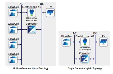 Figure 1. Hybrid photovoltaic-diesel generator microgrid topologies.
This work focused on analyzing a microgrid as applied to a small residential neighborhood. The demand profile for this was developed based on analysis of prior work and capabilities available within the HOMER software package to develop a realistic residential load profile. This profile was then scaled to approximate a neighborhood of 10-15 residential homes. Prior research has shown that residential load profiles exhibit lowest demand in the early hours of the morning, rise throughout the day with local peaks around hours six and twelve, and peak demand during the evening [20]. Load factors are typically very low for residential homes and approximated at 0.2 for this work. An example of this general residential load profile is shown in Figure 2. Variations from month to month, from day to day, and from time step to time step were modeled to further develop this into a more realistic representation of a small community load profile. More specifically, the data was varied ±10% day-to-day and ±20% from time-step-to-time-step. Additionally, seasonal variation was incorporated. Details on the final load profile are shown in the box-and-whisker plot in Figure 3 on a month by month basis. Peak loading in the summer is representative of expected air conditioner loads during that time. The final scaled load model for this work had an average energy consumption of 200 kWh/d with a peak load of 42.49 kW. The effects of demand response were simulated by allocating a percentage of this load to be eligible for DR.
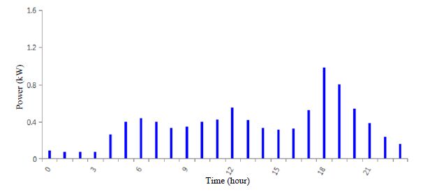 Figure 2. Sample hourly residential load profile.
 Figure 3. Monthly residential load.
Common loads that are candidates for DR, or can be deferred, include water pumps, water heaters, plug-in loads that are non-critical or have internal battery storage, and HVAC systems as discussed in [16]. The DR model used in this work allows for a designated load to be deferred in time. A generalized model for deferrable loads treats each load as a unit of energy that must be met within a certain time period with an associated load profile. For example, a water heater must maintain a certain temperature within the tank. This tank can be viewed as a storage reservoir with a capacity in kWh. Energy can be put into the tank until the maximum temperature is reached (e.g. full capacity) and the load can be deferred until the minimum temperature is reached (e.g. minimum capacity). While this is occurring, the tank is serving the end user based on a specified profile (e.g. providing hot water) which consumes energy. To add energy to the tank a specific load profile, power over time, is modeled. The model used in this work generalizes this concept as a percentage of total load that is available for DR. More specifically, this is modeled based on specifying the daily energy that can be deferred (as a percentage of total daily energy consumption), effective storage capacity of deferred load (in kWh), and the minimum/peak deferred load pr ofile values (in kW). In simulation, the primary load is provided for at all times. The deferrable load is served within specified guidelines. The strategy used for providing energy to the deferrable load is as follows:
|
PDL,min≤PDL≤PDL,max if(PAC+PDG≥PL,prim)∨(EDL=0)PDL=0 otherwise |
(1) |
where
PDL:is the deferrable load demand in the current time step (kW)
PDL,min:is the minimum deferrable load demand (kW)
PDL,max:is the maximum deferrable load demand (kW)
PL,prim:is the primary load demand in the current time step (kW)
EDL:is the energy in the deferrable load tank at the end of the prior time step (kWh)
PAC:is the AC power output from the converter in the current time step (kW)
PDG:is the power rating of the diesel generator(s) (kW)
In other words, the deferred load is provided energy when it is available (generation exceeds primary load demand) or if the load can be deferred no longer as the energy in the load tank has reached zero. For this work, the deferrable load available, and peak power of deferrable load, was designated as a percentage of total load. Storage capacity was set to 25% of deferrable load. For example, if DR was set to 10% of the load, then the base load was reduced to 180 kWh/d and 38.24 kW peak while the deferrable load was 20 kWh/d and 4.25 kW peak. Sensitivity analysis was performed on all the deferrable load parameters and minimal change in system performance was observed with the exception of energy available for deferment. As a result, the data presented in this paper focuses on system performance and economics as the quantity of deferrable load increases and holds other parameters fixed.
Solar PV generation has two key components to the model: solar resources available and the PV system energy conversion. Solar resource estimation was obtained from the National Solar Radiation Data Base [21] based on the geographical location of the system. A clearness index and solar radiation profile for various locations are available in this database. For this work the solar resources for Denver, Colorado, were used and can be seen in Figure 4. Denver was used as the location because the solar resources are fairly good (~ 5.5 kWh/m2/day average) and exhibits a good location for a hybrid microgrid with PV. The HOMER software used this data and models for the PV panels and inverter to determine how much PV power is generated at every time step of the simulation. More specifically, the AC power output from the PV array/converter combination was calculated at each time step by:
|
PAC=PDC,STCfPV(¯GT¯GT,STC)[1+α(¯Tc−¯Tc,STC)]ηconv |
(2) |
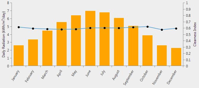 Figure 4. Monthly average solar global horizontal irradiance data and clearness index.
where
PAC:is the AC power output from the converter in the current time step (kW)
PDC,STC:is the DC power rating of the PV array under standard test conditions (kW)
fPV:is the PV derating factor to account for shading, system losses, soiling, ageing, etc. (%)
¯GT:is the average solar radiation incident on the PV array in the current time step (kW/m2)
¯GT,STC:is the average solar radiation incident on the PV array under STC (kW/m2)
α:is the temperature coefficient of power for the PV array (%/°C)
¯Tc:is average PV cell temperature in the current time step (°C)
¯Tc,STC:is the PV cell temperature under STC (°C)
ηconv:is the power electronic converter efficiency (%)
It is assumed that a maximum power point tracking converter is used. ¯GT was calculated based on panel orientation (latitude tilt, south facing in this work). Temperature data was imported from the surface meteorology and solar energy database [22]. Parameters for the PV panels and converter were chosen based off standard, commercially available, PV panels and converters. PV panel efficiency was 13%, nominal operating cell temperature 47 °C, derating factor 80%, and temperature coefficient −0.5%/°C. The inverter efficiency was 90%.
The diesel generator model was developed based on fuel data from commercially available diesel generators [23]. The generators studied in this work varied from 10-40 kW and, based on available data, exhibit very similar fuel/efficiency characteristics within this power range. Actual fuel consumption and efficiency can vary during operation and can also vary based on generator size, or brand/model of generator. However, the data used in this work is representative of commercially available diesel generators. The efficiency and fuel consumptions curves shown in Figure 5 and Figure 6 respectively are approximations of diesel generator performance in the range of 10-40 kW. The operational range of the generators were limited between 20-100% loading, shown by the shaded region in the figures, to increase generator efficiency and prevent wet stacking.
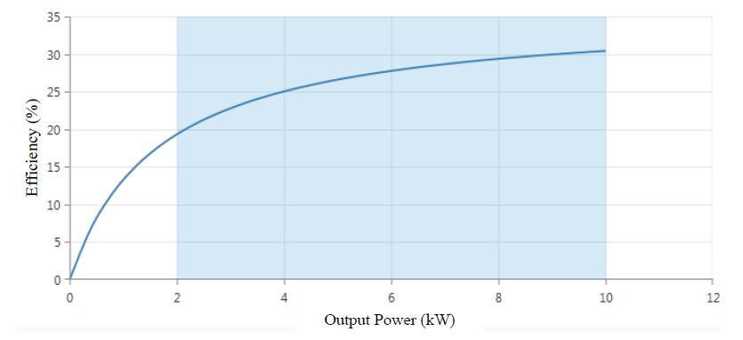 Figure 5. Diesel generator efficiency curve.
 Figure 6. Diesel generator fuel curve.
The systems shown in Figure 1 were constructed in HOMER and simulated for six different cases. More specifically, a base case with no DR, and five subsequent cases with DR increased by 10% each case for a maximum of 50% of the load available for DR. The time step was ten minutes and a simulation of twenty-five years was conducted for each case. For each time step an energy balance calculation is performed and flows of energy to and from each components of the system is determined. Energy production, energy consumption, diesel fuel consumption, system operating and O&M costs, etc. are calculated at each time step. Additionally, specified constraints are held during all time steps. For this work, 100% of load is served, a 10% operating reserve and 20% minimum loading constraints were placed on the generators, and a 0% capacity shortage constraint was set. System configurations that fail to meet these constraints were discarded as infeasible. This ensured that all loads would be met and some excess generation capacity is available at all times. Cost effectiveness of all feasible designs is compared in the simulation. The optimal solution, based on lowest cost of energy, is selected as the design choice for each case and was used to compare to other cases with different DR levels. System component costs, both capital and operation and maintenance costs, are enumerated in Table 1. These costs were estimat ed based on current installed and operational pricing of generators, converters, and PV panels at the time of this writing. The PV panels are expected to last the duration of the simulation time period, while the converter will need to be replaced after approximately fifteen years, and the generator after approximately 15, 000 hours of operation.
| Component | Capital Cost | Operation and Maintenance Cost |
| Diesel Generator | $500/kW | $0.03/hr + |
| $500/kW/15000hr replacement | ||
| Diesel Fuel | --- | $0.76/L |
| Photovoltaic Source | $3000/kW | $10/kW/yr |
| Power Electronic Converter | $400/kW | $300/kW/15yr replacement |
 DownLoad: CSV
The search space for system configurations included a wide range of PV and converter capacity in 5 kW increments and a wide range of diesel generator capacity in 10 kW increments. Each simulation was checked to ensure the optimal solution did not fall at the edge of the search space. The simulation results include the cost of energy (COE) in $/kWh, capital and operating costs, and diesel generator fuel consumption and hours of operation for each system configuration studied. A summary of these results are shown in Table 2 for the multiple generator base case (no DR). The optimal solution is shown at the top with a COE of $0.371/kWh in this case. A detailed analysis of energy production and consumption was also obtained and is shown in Figure 7. This case had 31% of the load supplied by the PV source and required four 10 kW diesel generators. Note that 7189.3 kWh/yr of excess electricity is generated. The excess generation is due to the minimum loading requirements on diesel generator sets to avoid wet stacking. More specifically, regardless of demand, a certain minimum loading of the diesel generators is required for reliability purposes. As a result, in some cases this minimum loading results in excess energy production. This excess energy can be routed into a dump load to maintain a minimum loading on the generator and/or PV generation can be curtailed to increa se generator loading. A detailed analysis of energy production and consumption for the base case with a single generator is shown in Figure 8. The next section provides simulation results on DR impacts in the hybrid microgrids shown in Figure 1.
| PV Capacity (kW) | Generator (kW) | Converter (kW) | COE ($) | Initial Capital ($) | Renewable Fraction (%) | 10kW Gen1 Fuel (L) | 10kW Gen2 Fuel (L) | 10kW Gen3 Fuel (L) | 10kW Gen4 Fuel (L) |
| 20 | 40 | 15 | 0.371 | 86000 | 31 | 15085 | 3272 | 674 | 97 |
| 25 | 40 | 15 | 0.372 | 101000 | 34 | 14176 | 3189 | 672 | 96 |
| 20 | 40 | 20 | 0.374 | 88000 | 31 | 15078 | 3272 | 674 | 97 |
| 25 | 40 | 20 | 0.374 | 103000 | 35 | 14116 | 3189 | 672 | 96 |
| 15 | 40 | 10 | 0.375 | 69000 | 25 | 16497 | 3394 | 682 | 98 |
| 20 | 40 | 10 | 0.375 | 84000 | 30 | 15484 | 3278 | 674 | 97 |
| 15 | 40 | 15 | 0.377 | 71000 | 26 | 16441 | 3394 | 682 | 98 |
| 15 | 40 | 20 | 0.379 | 73000 | 26 | 16441 | 3394 | 682 | 98 |
| 25 | 40 | 10 | 0.382 | 99000 | 32 | 14883 | 3200 | 672 | 96 |
| 10 | 40 | 10 | 0.383 | 54000 | 18 | 18055 | 3626 | 687 | 99 |
| 10 | 40 | 15 | 0.385 | 56000 | 18 | 18055 | 3626 | 687 | 99 |
| 10 | 40 | 5 | 0.386 | 52000 | 17 | 18405 | 3694 | 687 | 99 |
| 10 | 40 | 20 | 0.388 | 58000 | 18 | 18055 | 3626 | 687 | 99 |
| 15 | 40 | 5 | 0.394 | 67000 | 20 | 17869 | 3547 | 682 | 98 |
| 20 | 40 | 5 | 0.405 | 82000 | 21 | 17568 | 3463 | 674 | 97 |
| 25 | 40 | 5 | 0.419 | 97000 | 22 | 17395 | 3393 | 672 | 96 |
DownLoad: CSV Figure 7. Energy production and consumption results for multiple generator base case.
 Figure 8. Energy production and consumption results for single generator base case.
The simulation results for the single generator system are shown in Table 3 and Table 3. Table 4shows the optimal system configuration in regards to PV, Converter, and generator capacity over a wide range of DR (0-50%). As more load is available for DR, the capacity of all components is reduced. This effectively reduces system cost and improves the utilization of all system resources. This can be more clearly seen from the data in Table 4. For the base case scenario, there exists much excess electricity production (43, 421 kWh/yr) and only 13.5% of the consumed energy is provided for by the PV source. The COE for this base case is $0.657/kWh. Dramatic improvements are seen at any level of DR as COE, Fuel consumption, excess electricity production all decrease and renewable energy fraction increases as compared to the base case. At modest level of 20% of DR load, COE has been reduced by 21.16%, fuel consumption reduced by 16.74%, and excess electricity reduced by 75.39% as shown in Table 5. Generally speaking, system performance improves as DR increases. The primary impact of incorporating DR is the reduction of generation capacity, both PV and diesel, which is possible due to better utilization of these resources. This can be seen in the large jumps in performance between 10% and 20% DR, and 30% and 40% DR as capacity changes occur for optimal configurations. Simulation results for the multiple generator system are shown in Tables 6 and 7. Table 6 shows the optimal system configuration as DR capability varies. A similar trend in reduction of diesel generator capacity is seen. PV capacity increased as DR is increased as the flexibility of operating four generators allows for better utilization of PV as compared to the single generator case. Also note that the initial starting point is much more economical in comparison to the single generator system. The data in Table 7shows that appreciable reduction in COE and excess electricity production is achieved with DR while the renewable energy fraction and fuel consumption improvements are also seen. These results are significant but not as substantial as compared to the single generator case. The differences between the two cases are due solely to the generation architecture. At a modest level of 20% of DR load, COE has been reduced by 6.20%, fuel consumption reduced by 6.89%, and excess electricity reduced by 57.10% as shown in Table 8. As before, the primary impacts of DR are the reduction of diesel generation capacity, better utilization of all generation resources.
| Percentage of Load Available for DR | PV Capacity (kW) | Converter Capacity (kW) | Diesel Generator Capacity (kW) |
| 0% | 35 | 20 | 40 |
| 10% | 35 | 20 | 40 |
| 20% | 25 | 15 | 30 |
| 30% | 25 | 15 | 30 |
| 40% | 30 | 20 | 20 |
| 50% | 20 | 15 | 20 |
DownLoad: CSV| Percentage of Load Available for DR | Cost of Energy | Fuel Consumption | Excess Electricity Production | Renewable Energy Fraction |
| 0% | $0.657/kWh | 28,601 L | 43,421 kWh/yr | 13.5% |
| 10% | $0.653/kWh | 28,805 L | 39,230 kWh/yr | 19.0% |
| 20% | $0.518/kWh | 23,813 L | 14,555 kWh/yr | 31.0% |
| 30% | $0.499/kWh | 22,487 L | 10,684 kWh/yr | 36.0% |
| 40% | $0.397/kWh | 17,087 L | 11,169 kWh/yr | 45.4% |
| 50% | $0.383/kWh | 17,493 L | 4649 kWh/yr | 43.5% |
DownLoad: CSV| Percentage of Load Available for DR | Cost of Energy Reduction | Diesel Fuel Reduction | Excess Electricity Reduction |
| 10% | 0.61% | -0.71% | 9.65% |
| 20% | 21.16% | 16.74% | 66.48% |
| 30% | 24.05% | 21.38% | 75.39% |
| 40% | 39.57% | 40.26% | 74.28% |
| 50% | 41.70% | 38.84% | 89.29% |
DownLoad: CSV| Percentage of Load Available for DR | PV Capacity (kW) | Converter Capacity (kW) | Diesel Generator Capacity (kW) |
| 0% | 20 | 15 | 40 |
| 10% | 20 | 15 | 40 |
| 20% | 20 | 15 | 30 |
| 30% | 25 | 15 | 30 |
| 40% | 25 | 15 | 30 |
| 50% | 25 | 15 | 20 |
DownLoad: CSV| Percentage of Load Available for DR | Cost of Energy | Fuel Consumption | Excess Electricity Production | Renewable Energy Fraction |
| 0% | $0.371/kWh | 19,128 L | 7189 kWh/yr | 31.0% |
| 10% | $0.358/kWh | 18,270 L | 6034 kWh/yr | 33.9% |
| 20% | $0.348/kWh | 17,810 L | 3084 kWh/yr | 35.6% |
| 30% | $0.341/kWh | 16,241 L | 6626 kWh/yr | 41.1% |
| 40% | $0.335/kWh | 15,887 L | 5559 kWh/yr | 42.4% |
| 50% | $0.320/kWh | 15,314 L | 4607 kWh/yr | 43.6% |
DownLoad: CSV| Percentage of Load Available for DR | Cost of Energy Reduction | Diesel Fuel Reduction | Excess Electricity Reduction |
| 10% | 3.50% | 4.49% | 38.46% |
| 20% | 6.20% | 6.89% | 57.10% |
| 30% | 8.09% | 15.09% | 7.84% |
| 40% | 9.70% | 16.94% | 22.68% |
| 50% | 13.75% | 19.94% | 35.92% |
DownLoad: CSVSensitivity analysis was performed on solar resources and diesel fuel pricing to see how these affected the impacts of DR, energy pricing, and system configuration. Average solar insolation was varied between 4.0 and 6.5 kWh/m2/day and diesel fuel price was varied between $0.56 and $1.26 per liter. Base case results for the single generator system are shown in Figure 9 and Figure 10 while results for the single generator case with 20% DR are shown in Figure 11 and Figure 12. Figure 9 and Figure 11 provide data on excess electricity and COE, while Figure 10 and Figure 12 highlight renewable energy fraction across the range of solar irradiation and diesel fuel prices simulated. The impacts of DR in terms of COE, excess electricity, and renewable energy fraction were very similar over the simulated range of diesel fuel prices and solar resources. In regards to system configuration, the diesel generator sizes remained at 40 kW and 30 kW for the base case and 20% DR case respectively for all simulations. However, the PV/inverter capacities did change inversely proportional to solar insolation and directly proportional to diesel fuel price. In other words, the PV capacity can be decreased with better solar resources and increased in scenarios with higher fuel prices. In summary, these results indicate that the impact of DR will be very positive under a wide range of fuel prices and solar resource levels.
 Figure 9. Sensitivity analysis results showing excess electricity and COE for single generator base case.
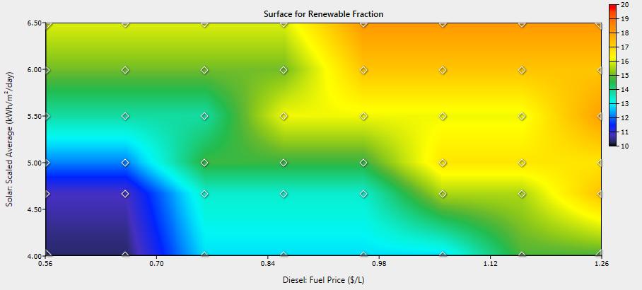 Figure 10. Sensitivity analysis results showing renewable energy fraction for single generator base case.
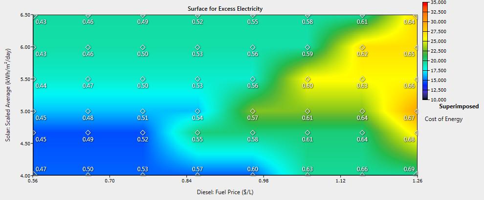 Figure 11. Sensitivity analysis results showing excess electricity and COE for single generator system with 20% DR.
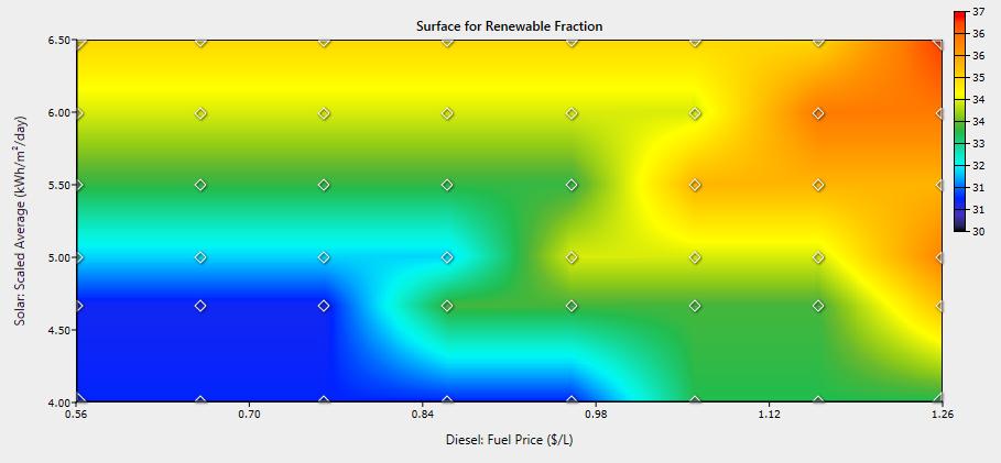 Figure 12. Sensitivity analysis results showing renewable energy fraction for single generator system with 20% DR.
Sensitivity analysis was performed on solar resources and diesel fuel pricing to see how these affected the impacts of DR, energy pricing, and system configuration. Average solar insolation was varied between 4.0 and 6.5 kWh/m2/day and diesel fuel price was varied between $0.56 and $1.26 per liter. Base case results for the single generator system are shown in Figure 9 and Figure 10 while results for the single generator case with 20% DR are shown in Figures 11 and 12. Figure 9 and provide data on excess electricity and COE, while Figures 10 and 12 highlight renewable energy fraction across the range of solar irradiation and diesel fuel prices simulated. The impacts of DR in terms of COE, excess electricity, and renewable energy fraction were very similar over the simulated range of diesel fuel prices and solar resources. In regards to system configuration, the diesel generator sizes remained at 40 kW and 30 kW for the base case and 20% DR case respectively for all simulations. However, the PV/inverter capacities did change inversely proportional to solar insolation and directly proportional to diesel fuel price. In other words, the PV capacity can be decreased with better solar resources and increased in scenarios with higher fuel prices. In summary, these results indicate that the impact of DR will be very positive under a wide range of fuel prices and solar resource levels.
The analysis in this paper focused on demand response impacts in off-grid hybrid PV-diesel generator microgrids as applied to a small residential community. System topologies with a single diesel generator and multiple diesel generators with parallel operation were studied. The primary objective was to analyze the impacts of DR in the absence of energy storage (e.g. batteries). While elimination of energy storage will not be feasible in all microgrid cases, it simplifies system design and increases system operation and reliability. Additionally, it was advantageous to remove energy storage in this analysis to isolate the impacts of DR. The results shown here indicate that the DR can improve the utilization of energy sources, in particular the intermittent PV source, substantially. As a result, fast acting DR or load shedding can be a valuable tool in designing and implementing efficient hybrid microgrids. Large reductions in the cost of energy, linked to reductions in initial capital and operating costs, are observed in both topologies. The single generator system showed the most improvement as it does not exhibit the advantages of paralleling generators. As a result, aggressive demand response/load shedding schemes could be an alternative to a multiple generator system. Future studies will investigate this further and analyze the feasible limits of DR in this application.
This work analyzed the impacts of demand response in an off-grid hybrid microgrid, containing diesel and photovoltaic generation, as applied to a small residential neighborhood. Prior research has shown the hybrid approach to be economical in off-grid applications and this study was performed by simulating two different hybrid diesel generator-PV microgrid topologies, one with a single diesel generator and one with multiple paralleled diesel generators, with varying levels of demand response. A detailed model of each microgrid was developed along with a cost analysis, to include initial capital and O&M costs. HOMER software was used to perform time domain simulations for each case at ten minute intervals over a period of twenty-five years. These simulations determined the optimal system design, defined as lowest cost of energy, for each case and provide data to analyze the impacts of DR in each case. These impacts were quantified through cost of energy reduction, diesel fuel reduction, and increased utilization of the energy sources. The presented results indicate that a moderate level of demand response can have significant positive impacts to the operation of hybrid microgrids as compared to a base case without demand response. For the single generator system and 20% of the load available for demand response, the cost of energy is reduced by 21.16%, fuel consumption reduced by 16.74%, and excess electricity reduced by 75.39%. For the multiple generator system and 20% of the load available for demand response, the cost of energy has been reduced by 6.20%, fuel consumption reduced by 6.89%, and excess electricity reduced by 57.10%. Sensitivity analysis showed that similar results can be expected across a wide range of solar resource levels and diesel fuel prices.
All authors declare no conflicts of interest in this paper.
| [1] |
Lemmens VEPP, Oenema A, Klepp KI, et al. (2008) A systematic review of the evidence regarding efficacy of obesity prevention interventions among adults. Obes Rev 9: 446-455. doi: 10.1111/j.1467-789X.2008.00468.x

|
| [2] | Shaw K, O'Rourke P, Del Mar C, et al. (2005) Psychological interventions for overweight or obesity. Cochrane Database Syst Rev: CD003818. |
| [3] |
Swinburn B, Egger G, Raza F (1999) Dissecting obesogenic environments: the development and application of a framework for identifying and prioritizing environmental interventions for obesity. Prev Med 29: 563-570. doi: 10.1006/pmed.1999.0585
|
| [4] |
McLaren L (2007) Socioeconomic status and obesity. Epidemiol Rev 29: 29-48. doi: 10.1093/epirev/mxm001
|
| [5] | Block JP, Scribner RA, DeSalvo KB (2004) Fast food, race/ethnicity, and income: a geographic analysis. Am J Prev Med 27: 211-217. |
| [6] |
Cummins SCJ, McKay L, MacIntyre S (2005) McDonald's restaurants and neighborhood deprivation in Scotland and England. Am J Prev Med 29: 308-310. doi: 10.1016/j.amepre.2005.06.011
|
| [7] |
Zenk SN, Schulz AJ, Israel BA, et al. (2005) Neighborhood racial composition, neighborhood poverty, and the spatial accessibility of supermarkets in metropolitan Detroit. Am J Public Health 95: 660-667. doi: 10.2105/AJPH.2004.042150
|
| [8] |
Smith DM, Cummins S, Taylor M, et al. (2010) Neighbourhood food environment and area deprivation: spatial accessibility to grocery stores selling fresh fruit and vegetables in urban and rural settings. Int J Epidemiol 39: 277-284. doi: 10.1093/ije/dyp221
|
| [9] |
Powell LM, Slater S, Mirtcheva D, et al. (2007) Food store availability and neighborhood characteristics in the United States. Prev Med 44: 189-195. doi: 10.1016/j.ypmed.2006.08.008
|
| [10] | Black C, Moon G, Baird J (2013) Dietary inequalities: What is the evidence for the effect of the neighbourhood food environment? Health Place. |
| [11] | Beaulac J, Kristjansson E, Cummins S (2009) A systematic review of food deserts, 1966-2007. Prev Chron Dis 6: A105. |
| [12] |
Black JL, Macinko J (2008) Neighborhoods and obesity. Nutr Rev 66: 2-20. doi: 10.1111/j.1753-4887.2007.00001.x
|
| [13] |
Larson NI, Story MT, Nelson MC (2009) Neighborhood environments disparities in access to healthy foods in the U.S. Am J Prev Med 36: 74-81. doi: 10.1016/j.amepre.2008.09.025
|
| [14] |
Walker RE, Keane CR, Burke JG (2010) Disparities and access to healthy food in the United States: A review of food deserts literature. Health Place 16: 876-884. doi: 10.1016/j.healthplace.2010.04.013
|
| [15] |
Fleischhacker SE, Evenson KR, Rodriguez DA, et al. (2011) A systematic review of fast food access studies. Obes Rev 12: e460-e471. doi: 10.1111/j.1467-789X.2010.00715.x
|
| [16] |
Fraser LK, Edwards KL, Cade J, et al. (2010) The geography of fast food outlets: a review. Int J Environ Res Publ Health 7: 2290-2308. doi: 10.3390/ijerph7052290
|
| [17] |
Hilmers A, Hilmers DC, Dave J (2012) Neighborhood disparities in access to healthy foods and their effects on environmental justice. Am J Public Health 102: 1644-1654. doi: 10.2105/AJPH.2012.300865
|
| [18] |
Ford PB, Dzewaltowski DA (2008) Disparities in obesity prevalence due to variation in the retail food environment: three testable hypotheses. Nutr Rev 66: 216-228. doi: 10.1111/j.1753-4887.2008.00026.x
|
| [19] |
Wells CS, Hintze JM (2007) Dealing with assumptions underlying statistical tests. Psychol Schools 44: 495-502. doi: 10.1002/pits.20241
|
| [20] |
Havlicek LL, Peterson NL (1974) Robustness of t test - a guide for researchers on effect of violations of assumptions. Psychol Rep 34: 1095-1114. doi: 10.2466/pr0.1974.34.3c.1095
|
| [21] |
Burgoine T, Alvanides S, Lake AA (2013) Creating‘obesogenic realities’; do our methodological choices make a difference when measuring the food environment? Int J Health Geogr 12: 33. doi: 10.1186/1476-072X-12-33
|
| [22] | Fotheringham AS, Brunsdon C, Charlton M (2002) Geographically weighted regression: the analysis of spatially varying relationships: Chichester, England: John Wiley, 2002. |
| [23] |
Glanz K, Sallis JF, Saelens BE, et al. (2005) Healthy nutrition environments: concepts and measures. Am J Health Promot 19: 330-333, ii. doi: 10.4278/0890-1171-19.5.330
|
| [24] | Holsten JE (2009) Obesity and the community food environment: a systematic review. Public Health Nutr 12: 397-405. |
| [25] |
Lennon JJ (2000) Red-shifts and red herrings in geographical ecology. Ecography 23: 101-113. doi: 10.1111/j.1600-0587.2000.tb00265.x
|
| [26] | Dale MRT, Fortin MJ (2002) Spatial autocorrelation and statistical tests in ecology. Ecoscience 9: 162-167. |
| [27] |
Chi G, Zhu J (2008) Spatial regression models for demographic analysis. Popul Res Policy Rev 27: 17-42. doi: 10.1007/s11113-007-9051-8
|
| [28] |
Dormann CF (2007) Effects of incorporating spatial autocorrelation into the analysis of species distribution data. Global Ecol Biogeogr 16: 129-138. doi: 10.1111/j.1466-8238.2006.00279.x
|
| [29] | Cushon J, Creighton T, Kershaw T, et al. (2013) Deprivation and food access and balance in Saskatoon, Saskatchewan. Chronic Dis Inj Can 33: 146-159. |
| [30] |
Lee G, Lim H (2009) A spatial statistical approach to identifying areas with poor access to grocery foods in the city of Buffalo, New York. Urban Stud 46: 1299-1315. doi: 10.1177/0042098009104567
|
| [31] |
Schneider S, Gruber J (2013) Neighbourhood deprivation and outlet density for tobacco, alcohol and fast food: first hints of obesogenic and addictive environments in Germany. Public Health Nutr 16: 1168-1177. doi: 10.1017/S1368980012003321
|
| [32] |
Bower KM, Thorpe RJ, Jr., Rohde C, et al. (2014) The intersection of neighborhood racial segregation, poverty, and urbanicity and its impact on food store availability in the United States. Prev Med 58: 33-39. doi: 10.1016/j.ypmed.2013.10.010
|
| [33] |
Thornton L, Pearce J, Kavanagh A (2011) Using Geographic Information Systems (GIS) to assess the role of the built environment in influencing obesity: a glossary. Int J Behav Nutr Phys Act 8: 71. doi: 10.1186/1479-5868-8-71
|
| [34] |
Moore LV, Diez Roux AV (2006) Associations of neighborhood characteristics with the location and type of food stores. Am J Public Health 96: 325-331. doi: 10.2105/AJPH.2004.058040
|
| [35] |
Anchondo TM, Ford PB (2011) Neighborhood deprivation, neighborhood acculturation, and the retail food environment in a US-Mexico border urban area. J Hunger Environ Nutr 6: 207-219. doi: 10.1080/19320248.2011.576214
|
| [36] |
Morland K, Wing S, Diez Roux A, et al. (2002) Neighborhood characteristics associated with the location of food stores and food service places. Am J Prev Med 22: 23-29. doi: 10.1016/S0749-3797(01)00403-2
|
| [37] |
Powell LA, Chaloupka FJ, Bao Y (2007) The availability of fast-food and full-service restaurants in the United States - Associations with neighborhood characteristics. Am J Prev Med 33: S240-S245. doi: 10.1016/j.amepre.2007.07.005
|
| [38] | Hurvitz PM, Moudon AV, Rehm CD, et al. (2009) Arterial roads and area socioeconomic status are predictors of fast food restaurant density in King County, WA. Int J Behav Nutr Phys Act 6. |
| [39] |
Kawakami N, Winkleby M, Skog L, et al. (2011) Differences in neighborhood accessibility to health-related resources: A nationwide comparison between deprived and affluent neighborhoods in Sweden. Health Place 17: 132-139. doi: 10.1016/j.healthplace.2010.09.005
|
| [40] |
Black JL, Carpiano RM, Fleming S, et al. (2011) Exploring the distribution of food stores in British Columbia: associations with neighbourhood socio-demographic factors and urban form. Health Place 17: 961-970. doi: 10.1016/j.healthplace.2011.04.002
|
| [41] |
Svastisalee CM, Nordah H, Glumer C, et al. (2011) Supermarket and fast-food outlet exposure in Copenhagen: associations with socio-economic and demographic characteristics. Public Health Nutr 14: 1618-1626. doi: 10.1017/S1368980011000759
|
| [42] |
Molaodi OR, Leyland AH, Ellaway A, et al. (2012) Neighbourhood food and physical activity environments in England, UK: Does ethnic density matter? Int J Behav Nutr Phys Act 9: 75. doi: 10.1186/1479-5868-9-75
|
| [43] |
Lisabeth LD, Sanchez BN, Escobar J, et al. (2010) The food environment in an urban Mexican American community. Health Place 16: 598-605. doi: 10.1016/j.healthplace.2010.01.005
|
| [44] |
Kwate NO, Yau CY, Loh JM, et al. (2009) Inequality in obesigenic environments: fast food density in New York City. Health Place 15: 364-373. doi: 10.1016/j.healthplace.2008.07.003
|
| [45] | Baker EA, Schootman M, Barnidge E, et al. (2006) The role of race and poverty in access to foods that enable individuals to adhere to dietary guidelines. Prev Chronic Dis 3: A76. |
| [46] |
Jaime PC, Duran AC, Sarti FM, et al. (2011) Investigating environmental determinants of diet, physical activity, and overweight among adults in Sao Paulo, Brazil. J Urban Health 88: 567-581. doi: 10.1007/s11524-010-9537-2
|
| [47] |
Macintyre S, McKay L, Cummins S, et al. (2005) Out-of-home food outlets and area deprivation: case study in Glasgow, UK. Int J Behav Nutr Phys Act 2: 16. doi: 10.1186/1479-5868-2-16
|
| [48] |
Apparicio P, Cloutier MS, Shearmur R (2007) The case of Montréal's missing food deserts: evaluation of accessibility to food supermarkets. Int J Health Geogr 6: 4. doi: 10.1186/1476-072X-6-4
|
| [49] | Sharkey JR, Horel S, Han D, et al. (2009) Association between neighborhood need and spatial access to food stores and fast food restaurants in neighborhoods of colonias. Int J Health Geogr 8. |
| [50] | Hill JL, Chau C, Luebbering CR, et al. (2012) Does availability of physical activity and food outlets differ by race and income? Findings from an enumeration study in a health disparate region. Int J Behav Nutr Phys Act 9. |
| [51] |
Howard PH, Fulfrost B (2007) The density of retail food outlets in the central coast region of California: associations with income and Latino ethnic composition. J Hunger Environ Nutr 2: 3-18. doi: 10.1080/19320240802077789
|
| [52] |
Ball K, Timperio A, Crawford D (2009) Neighbourhood socioeconomic inequalities in food access and affordability. Health Place 15: 578-585. doi: 10.1016/j.healthplace.2008.09.010
|
| [53] |
Pearce J, Blakely T, Witten K, et al. (2007) Neighborhood deprivation and access to fast-food retailing: A national study. Am J Prev Med 32: 375-382. doi: 10.1016/j.amepre.2007.01.009
|
| [54] |
Pearce J, Witten K, Hiscock R, et al. (2007) Are socially disadvantaged neighbourhoods deprived of health-related community resources? Int J Epidemiol 36: 348-355. doi: 10.1093/ije/dyl267
|
| [55] |
Pearce J, Witten K, Hiscock R, et al. (2008) Regional and urban-rural variations in the association of neighbourhood deprivation with community resource access: a national study. Environ Plann A 40: 2469-2489. doi: 10.1068/a409
|
| [56] |
Smoyer-Tomic KE, Spence JC, Raine KD, et al. (2008) The association between neighborhood socioeconomic status and exposure to supermarkets and fast food outlets. Health Place 14: 740-754. doi: 10.1016/j.healthplace.2007.12.001
|
| [57] |
Burns CM, Inglis AD (2007) Measuring food access in Melbourne: access to healthy and fast foods by car, bus and foot in an urban municipality in Melbourne. Health Place 13: 877-885. doi: 10.1016/j.healthplace.2007.02.005
|
| [58] |
Cubbin C, Jun J, Margerison-Zilko C, et al. (2012) Social inequalities in neighborhood conditions: spatial relationships between sociodemographic and food environments in Alameda County, California. Journal of Maps 8: 344-348. doi: 10.1080/17445647.2012.747992
|
| [59] |
Dai D, Wang F (2011) Geographic disparities in accessibility to food stores in Southwest Mississippi. Environ Plann B 38: 659-677. doi: 10.1068/b36149
|
| [60] | Larch M, Walde J (2008) Lag or error? - Detecting the nature of spatial correlation. In: Preisach C, Burkhardt H, Schmidt-Thieme L et al., editors. Data analysis, machine learning and applications: Springer Berlin Heidelberg. pp. 301-308. |
| [61] | Anselin L (2001) A companion to theoretical econometrics. Chapter 14: Spatial econometrics; Baltagi BH, editor. Malden, MA: Blackwell Publishing Ltd. |
| [62] | Getis A, Ord JK (1992) The analysis of spatial association by use of distance statistics. Geogr Anal 24: 189-206. |
| [63] |
Bader MDM, Purciel M, Yousefzadeh P, et al. (2010) Disparities in neighborhood food environments: implications of measurement strategies. Econ Geogr 86: 409-430. doi: 10.1111/j.1944-8287.2010.01084.x
|
| [64] |
Berg N, Murdoch J (2008) Access to grocery stores in Dallas. Int J Behav Healthc Res 1: 22-37. doi: 10.1504/IJBHR.2008.018449
|
| [65] | Daniel M, Kestens Y, Paquet C (2009) Demographic and urban form correlates of healthful and unhealthful food availability in Montréal, Canada. Can J Public Health 100: 189-193. |
| [66] |
Gordon C, Purciel-Hill M, Ghai NR, et al. (2011) Measuring food deserts in New York City's low-income neighborhoods. Health Place 17: 696-700. doi: 10.1016/j.healthplace.2010.12.012
|
| [67] | Gould AC, Apparicio P, Cloutier M-S (2012) Classifying neighbourhoods by level of access to stores selling fresh fruit and vegetables and groceries: identifying problematic areas in the city of Gatineau, Quebec. Can J Public Health 103: e433-e437. |
| [68] |
Hemphill E, Raine K, Spence JC, et al. (2008) Exploring obesogenic food environments in Edmonton, Canada: The association between socioeconomic factors and fast food outlet access. Am J Health Prom 22: 426-432. doi: 10.4278/ajhp.22.6.426
|
| [69] | Jones J, Terashima M, Rainham D (2009) Fast food and deprivation in Nova Scotia. Can J Public Health 100: 32-35. |
| [70] |
Larsen K, Gilliland J (2008) Mapping the evolution of ‘food deserts’ in a Canadian city: supermarket accessibility in London, Ontario, 1961-2005. Int J Health Geogr 7: 16. doi: 10.1186/1476-072X-7-16
|
| [71] |
Macdonald L, Cummins S, Macintyre S (2007) Neighbourhood fast food environment and area deprivation-substitution or concentration? Appetite 49: 251-254. doi: 10.1016/j.appet.2006.11.004
|
| [72] |
Macdonald L, Ellaway A, Macintyre S (2009) The food retail environment and area deprivation in Glasgow City, UK. Int J Behav Nutr Phys Act 6: 52. doi: 10.1186/1479-5868-6-52
|
| [73] | Macintyre S, Macdonald L, Ellaway A (2008) Do poorer people have poorer access to local resources and facilities? The distribution of local resources by area deprivation in Glasgow, Scotland. Soc Sci Med 67: 900-914. |
| [74] | Meltzer R, Schuetz J (2012) Bodegas or bagel shops? Neighborhood differences in retail and household services. Econ Devel Quart 26: 73-94. |
| [75] |
Mercille G, Richard L, Gauvin L, et al. (2013) Comparison of two indices of availability of fruits/vegetable and fast food outlets. J Urban Health 90: 240-245. doi: 10.1007/s11524-012-9722-6
|
| [76] |
Pearce J, Day P, Witten K (2008) Neighbourhood provision of food and alcohol retailing and social deprivation in urban New Zealand. Urban Policy Res 26: 213-227. doi: 10.1080/08111140701697610
|
| [77] |
Reidpath DD, Burns C, Garrard J, et al. (2002) An ecological study of the relationship between social and environmental determinants of obesity. Health Place 8: 141-145. doi: 10.1016/S1353-8292(01)00028-4
|
| [78] | Richardson AS, Boone-Heinonen J, Popkin BM, et al. (2012) Are neighbourhood food resources distributed inequitably by income and race in the USA? Epidemiological findings across the urban spectrum. BMJ Open 2: e000698. |
| [79] |
Rigby S, Leone AF, Hwahwan K, et al. (2012) Food deserts in Leon County, FL: Disparate distribution of supplemental nutrition assistance program-accepting stores by neighborhood characteristics. J Nutr Educ Behav 44: 539-547. doi: 10.1016/j.jneb.2011.06.007
|
| [80] | Sharkey JR, Horel S (2008) Neighborhood socioeconomic deprivation and minority composition are associated with better potential spatial access to the ground-truthed food environment in a large rural area. J Nutr 138: 620-627. |
| [81] |
Sharkey JR, Johnson CM, Dean WR, et al. (2011) Focusing on fast food restaurants alone underestimates the relationship between neighborhood deprivation and exposure to fast food in a large rural area. Nutr J 10: 10. doi: 10.1186/1475-2891-10-10
|
| [82] |
Lumley T, Diehr P, Emerson S, et al. (2002) The importance of the normality assumption in large public health data sets. Annu Rev Public Health 23: 151-169. doi: 10.1146/annurev.publhealth.23.100901.140546
|
| [83] |
Lamb KE, White SR (2015) Categorisation of built environment characteristics: the trouble with tertiles. Int J Behav Nutr Phys Act 12: 19. doi: 10.1186/s12966-015-0181-9
|
| [84] |
Lamb KE, Ogilvie D, Ferguson NS, et al. (2012) Sociospatial distribution of access to facilities for moderate and vigorous intensity physical activity in Scotland by different modes of transport. Int J Behav Nutr Phys Act 9: 55. doi: 10.1186/1479-5868-9-55
|
| [85] |
Ogilvie D, Lamb KE, Ferguson NS, et al. (2011) Recreational physical activity facilities within walking and cycling distance: Sociospatial patterning of access in Scotland. Health Place 17: 1015-1022. doi: 10.1016/j.healthplace.2011.07.003
|
| [86] | Littell RC, Milliken GA, Stroup WW, et al. (2006) SAS® for mixed models: SAS Institute. |
| [87] | Drukker DM, Prucha IR, Raciborski R (2013) Maximum likelihood and generalized spatial two-stage least-squares estimators for a spatial-autoregressive model with spatial-autoregressive disturbances. The Stata Journal 13: 221-241. |
| [88] | Drukker DM, Peng H, Prucha IR, et al. (2013) Creating and managing spatial-weighting matrices with the spmat command. The Stata Journal 13: 242-286. |
| [89] | Bivand R (2014) spdep: Spatial dependence: weighting schemes, statistics and models. R package version 0.5-74 http://CRAN.R-project.org/package=spdep. |
| [90] |
Anselin L, Syabri I, Kho Y (2006) GeoDa: An introduction to spatial data analysis. Geogr Anal 38: 5-22. doi: 10.1111/j.0016-7363.2005.00671.x
|
| [91] | Kaluzny SP, Vega SC, Cardoso TP, et al. (1998) S+ SpatialStats user's manual for Windows and UNIX.; SolutionMetrics Pty Ltd, editor. New York: Springer. |
| [92] |
Pace RK, Barry R (1997) Sparse spatial autoregressions. Stat Probabil Lett 33: 291-297. doi: 10.1016/S0167-7152(96)00140-X
|
| [93] |
Walde J, Larch M, Tappeiner G (2008) Performance contest between MLE and GMM for huge spatial autoregressive models. J Stat Comput Sim 78: 151-166. doi: 10.1080/10629360600954109
|
| [94] | Fortin M-J, Dale MRT (2005) Spatial analysis: a guide for ecologists: New York: Cambridge University Press, 2005. |
| [95] |
Kleinschmidt I, Sharp B, Mueller I, et al. (2002) Rise in malaria incidence rates in South Africa: a small-area spatial analysis of variation in time trends. Am J Epidemiol 155: 257-264. doi: 10.1093/aje/155.3.257
|
| [96] |
Rytkönen M, Moltchanova E, Ranta J, et al. (2003) The incidence of type 1 diabetes among children in Finland-rural–urban difference. Health Place 9: 315-325. doi: 10.1016/S1353-8292(02)00064-3
|
| [97] |
Salcedo N, Saez M, Bragulat B, et al. (2012) Does the effect of gender modify the relationship between deprivation and mortality? BMC Public Health 12: 574. doi: 10.1186/1471-2458-12-574
|
| [98] |
Gerstner K, Dormann CF, Václavík T, et al. (2014) Accounting for geographical variation in species–area relationships improves the prediction of plant species richness at the global scale. Journal of Biogeography 41: 261-273. doi: 10.1111/jbi.12213
|
| [99] | Pioz M, Guis H, Crespin L, et al. (2012) Why did bluetongue spread the way it did? Environmental factors influencing the velocity of bluetongue virus serotype 8 epizootic wave in France. PLoS One 7: e43360. |
| [100] |
Liebhold AM, McCullough DG, Blackburn LM, et al. (2013) A highly aggregated geographical distribution of forest pest invasions in the USA. Diversity and Distributions 19: 1208-1216. doi: 10.1111/ddi.12112
|
| [101] | Kissling WD, Carl G (2008) Spatial autocorrelation and the selection of simultaneous autoregressive models. Global Ecol Biogeogr 17: 59-71. |
| [102] |
Wall MM (2004) A close look at the spatial structure implied by the CAR and SAR models. J Stat Plan Infer 121: 311-324. doi: 10.1016/S0378-3758(03)00111-3
|
| [103] |
Mur J, Angulo AM (2007) Clues for discriminating between moving average and autoregressive models in spatial processes. Span Econ Rev 9: 273-298. doi: 10.1007/s10108-006-9018-7
|
| [104] |
Austin SB, Melly SJ, Sanchez BN, et al. (2005) Clustering of fast-food restaurants around schools: A novel application of spatial statistics to the study of food environments. Am J Public Health 95: 1575-1581. doi: 10.2105/AJPH.2004.056341
|
| [105] |
Spielman S (2006) Appropriate use of the K-function in urban environments. Am J Public Health 96: 205-205. doi: 10.2105/AJPH.2005.078857
|
| 1. | Henry Louie, Operational analysis of hybrid solar/wind microgrids using measured data, 2016, 31, 09730826, 108, 10.1016/j.esd.2016.01.003 | |
| 2. | Madison Stark, Aaron St. Leger, Nicholas Barry, 2018, Tactical generator monitoring system, 978-1-5386-1006-0, 1, 10.1109/TPEC.2018.8312095 |
Figures(1) / Tables(3)

Karen E. Lamb, Lukar E. Thornton, Ester Cerin, Kylie Ball. Statistical Approaches Used to Assess the Equity of Access to Food Outlets: A Systematic Review[J]. AIMS Public Health, 2015, 2(3): 358-401. doi: 10.3934/publichealth.2015.3.358

| Component | Capital Cost | Operation and Maintenance Cost |
| Diesel Generator | $500/kW | $0.03/hr + |
| $500/kW/15000hr replacement | ||
| Diesel Fuel | --- | $0.76/L |
| Photovoltaic Source | $3000/kW | $10/kW/yr |
| Power Electronic Converter | $400/kW | $300/kW/15yr replacement |
DownLoad: CSV| PV Capacity (kW) | Generator (kW) | Converter (kW) | COE ($) | Initial Capital ($) | Renewable Fraction (%) | 10kW Gen1 Fuel (L) | 10kW Gen2 Fuel (L) | 10kW Gen3 Fuel (L) | 10kW Gen4 Fuel (L) |
| 20 | 40 | 15 | 0.371 | 86000 | 31 | 15085 | 3272 | 674 | 97 |
| 25 | 40 | 15 | 0.372 | 101000 | 34 | 14176 | 3189 | 672 | 96 |
| 20 | 40 | 20 | 0.374 | 88000 | 31 | 15078 | 3272 | 674 | 97 |
| 25 | 40 | 20 | 0.374 | 103000 | 35 | 14116 | 3189 | 672 | 96 |
| 15 | 40 | 10 | 0.375 | 69000 | 25 | 16497 | 3394 | 682 | 98 |
| 20 | 40 | 10 | 0.375 | 84000 | 30 | 15484 | 3278 | 674 | 97 |
| 15 | 40 | 15 | 0.377 | 71000 | 26 | 16441 | 3394 | 682 | 98 |
| 15 | 40 | 20 | 0.379 | 73000 | 26 | 16441 | 3394 | 682 | 98 |
| 25 | 40 | 10 | 0.382 | 99000 | 32 | 14883 | 3200 | 672 | 96 |
| 10 | 40 | 10 | 0.383 | 54000 | 18 | 18055 | 3626 | 687 | 99 |
| 10 | 40 | 15 | 0.385 | 56000 | 18 | 18055 | 3626 | 687 | 99 |
| 10 | 40 | 5 | 0.386 | 52000 | 17 | 18405 | 3694 | 687 | 99 |
| 10 | 40 | 20 | 0.388 | 58000 | 18 | 18055 | 3626 | 687 | 99 |
| 15 | 40 | 5 | 0.394 | 67000 | 20 | 17869 | 3547 | 682 | 98 |
| 20 | 40 | 5 | 0.405 | 82000 | 21 | 17568 | 3463 | 674 | 97 |
| 25 | 40 | 5 | 0.419 | 97000 | 22 | 17395 | 3393 | 672 | 96 |
DownLoad: CSV| Percentage of Load Available for DR | PV Capacity (kW) | Converter Capacity (kW) | Diesel Generator Capacity (kW) |
| 0% | 35 | 20 | 40 |
| 10% | 35 | 20 | 40 |
| 20% | 25 | 15 | 30 |
| 30% | 25 | 15 | 30 |
| 40% | 30 | 20 | 20 |
| 50% | 20 | 15 | 20 |
DownLoad: CSV| Percentage of Load Available for DR | Cost of Energy | Fuel Consumption | Excess Electricity Production | Renewable Energy Fraction |
| 0% | $0.657/kWh | 28,601 L | 43,421 kWh/yr | 13.5% |
| 10% | $0.653/kWh | 28,805 L | 39,230 kWh/yr | 19.0% |
| 20% | $0.518/kWh | 23,813 L | 14,555 kWh/yr | 31.0% |
| 30% | $0.499/kWh | 22,487 L | 10,684 kWh/yr | 36.0% |
| 40% | $0.397/kWh | 17,087 L | 11,169 kWh/yr | 45.4% |
| 50% | $0.383/kWh | 17,493 L | 4649 kWh/yr | 43.5% |
DownLoad: CSV| Percentage of Load Available for DR | Cost of Energy Reduction | Diesel Fuel Reduction | Excess Electricity Reduction |
| 10% | 0.61% | -0.71% | 9.65% |
| 20% | 21.16% | 16.74% | 66.48% |
| 30% | 24.05% | 21.38% | 75.39% |
| 40% | 39.57% | 40.26% | 74.28% |
| 50% | 41.70% | 38.84% | 89.29% |
DownLoad: CSV| Percentage of Load Available for DR | PV Capacity (kW) | Converter Capacity (kW) | Diesel Generator Capacity (kW) |
| 0% | 20 | 15 | 40 |
| 10% | 20 | 15 | 40 |
| 20% | 20 | 15 | 30 |
| 30% | 25 | 15 | 30 |
| 40% | 25 | 15 | 30 |
| 50% | 25 | 15 | 20 |
DownLoad: CSV| Percentage of Load Available for DR | Cost of Energy | Fuel Consumption | Excess Electricity Production | Renewable Energy Fraction |
| 0% | $0.371/kWh | 19,128 L | 7189 kWh/yr | 31.0% |
| 10% | $0.358/kWh | 18,270 L | 6034 kWh/yr | 33.9% |
| 20% | $0.348/kWh | 17,810 L | 3084 kWh/yr | 35.6% |
| 30% | $0.341/kWh | 16,241 L | 6626 kWh/yr | 41.1% |
| 40% | $0.335/kWh | 15,887 L | 5559 kWh/yr | 42.4% |
| 50% | $0.320/kWh | 15,314 L | 4607 kWh/yr | 43.6% |
DownLoad: CSV| Percentage of Load Available for DR | Cost of Energy Reduction | Diesel Fuel Reduction | Excess Electricity Reduction |
| 10% | 3.50% | 4.49% | 38.46% |
| 20% | 6.20% | 6.89% | 57.10% |
| 30% | 8.09% | 15.09% | 7.84% |
| 40% | 9.70% | 16.94% | 22.68% |
| 50% | 13.75% | 19.94% | 35.92% |
DownLoad: CSV| Component | Capital Cost | Operation and Maintenance Cost |
| Diesel Generator | $500/kW | $0.03/hr + |
| $500/kW/15000hr replacement | ||
| Diesel Fuel | --- | $0.76/L |
| Photovoltaic Source | $3000/kW | $10/kW/yr |
| Power Electronic Converter | $400/kW | $300/kW/15yr replacement |
| PV Capacity (kW) | Generator (kW) | Converter (kW) | COE ($) | Initial Capital ($) | Renewable Fraction (%) | 10kW Gen1 Fuel (L) | 10kW Gen2 Fuel (L) | 10kW Gen3 Fuel (L) | 10kW Gen4 Fuel (L) |
| 20 | 40 | 15 | 0.371 | 86000 | 31 | 15085 | 3272 | 674 | 97 |
| 25 | 40 | 15 | 0.372 | 101000 | 34 | 14176 | 3189 | 672 | 96 |
| 20 | 40 | 20 | 0.374 | 88000 | 31 | 15078 | 3272 | 674 | 97 |
| 25 | 40 | 20 | 0.374 | 103000 | 35 | 14116 | 3189 | 672 | 96 |
| 15 | 40 | 10 | 0.375 | 69000 | 25 | 16497 | 3394 | 682 | 98 |
| 20 | 40 | 10 | 0.375 | 84000 | 30 | 15484 | 3278 | 674 | 97 |
| 15 | 40 | 15 | 0.377 | 71000 | 26 | 16441 | 3394 | 682 | 98 |
| 15 | 40 | 20 | 0.379 | 73000 | 26 | 16441 | 3394 | 682 | 98 |
| 25 | 40 | 10 | 0.382 | 99000 | 32 | 14883 | 3200 | 672 | 96 |
| 10 | 40 | 10 | 0.383 | 54000 | 18 | 18055 | 3626 | 687 | 99 |
| 10 | 40 | 15 | 0.385 | 56000 | 18 | 18055 | 3626 | 687 | 99 |
| 10 | 40 | 5 | 0.386 | 52000 | 17 | 18405 | 3694 | 687 | 99 |
| 10 | 40 | 20 | 0.388 | 58000 | 18 | 18055 | 3626 | 687 | 99 |
| 15 | 40 | 5 | 0.394 | 67000 | 20 | 17869 | 3547 | 682 | 98 |
| 20 | 40 | 5 | 0.405 | 82000 | 21 | 17568 | 3463 | 674 | 97 |
| 25 | 40 | 5 | 0.419 | 97000 | 22 | 17395 | 3393 | 672 | 96 |
| Percentage of Load Available for DR | PV Capacity (kW) | Converter Capacity (kW) | Diesel Generator Capacity (kW) |
| 0% | 35 | 20 | 40 |
| 10% | 35 | 20 | 40 |
| 20% | 25 | 15 | 30 |
| 30% | 25 | 15 | 30 |
| 40% | 30 | 20 | 20 |
| 50% | 20 | 15 | 20 |
| Percentage of Load Available for DR | Cost of Energy | Fuel Consumption | Excess Electricity Production | Renewable Energy Fraction |
| 0% | $0.657/kWh | 28,601 L | 43,421 kWh/yr | 13.5% |
| 10% | $0.653/kWh | 28,805 L | 39,230 kWh/yr | 19.0% |
| 20% | $0.518/kWh | 23,813 L | 14,555 kWh/yr | 31.0% |
| 30% | $0.499/kWh | 22,487 L | 10,684 kWh/yr | 36.0% |
| 40% | $0.397/kWh | 17,087 L | 11,169 kWh/yr | 45.4% |
| 50% | $0.383/kWh | 17,493 L | 4649 kWh/yr | 43.5% |
| Percentage of Load Available for DR | Cost of Energy Reduction | Diesel Fuel Reduction | Excess Electricity Reduction |
| 10% | 0.61% | -0.71% | 9.65% |
| 20% | 21.16% | 16.74% | 66.48% |
| 30% | 24.05% | 21.38% | 75.39% |
| 40% | 39.57% | 40.26% | 74.28% |
| 50% | 41.70% | 38.84% | 89.29% |
| Percentage of Load Available for DR | PV Capacity (kW) | Converter Capacity (kW) | Diesel Generator Capacity (kW) |
| 0% | 20 | 15 | 40 |
| 10% | 20 | 15 | 40 |
| 20% | 20 | 15 | 30 |
| 30% | 25 | 15 | 30 |
| 40% | 25 | 15 | 30 |
| 50% | 25 | 15 | 20 |
| Percentage of Load Available for DR | Cost of Energy | Fuel Consumption | Excess Electricity Production | Renewable Energy Fraction |
| 0% | $0.371/kWh | 19,128 L | 7189 kWh/yr | 31.0% |
| 10% | $0.358/kWh | 18,270 L | 6034 kWh/yr | 33.9% |
| 20% | $0.348/kWh | 17,810 L | 3084 kWh/yr | 35.6% |
| 30% | $0.341/kWh | 16,241 L | 6626 kWh/yr | 41.1% |
| 40% | $0.335/kWh | 15,887 L | 5559 kWh/yr | 42.4% |
| 50% | $0.320/kWh | 15,314 L | 4607 kWh/yr | 43.6% |
| Percentage of Load Available for DR | Cost of Energy Reduction | Diesel Fuel Reduction | Excess Electricity Reduction |
| 10% | 3.50% | 4.49% | 38.46% |
| 20% | 6.20% | 6.89% | 57.10% |
| 30% | 8.09% | 15.09% | 7.84% |
| 40% | 9.70% | 16.94% | 22.68% |
| 50% | 13.75% | 19.94% | 35.92% |
