


Citation: Theresa A. Nicklas, Carol E. O'Neil. Prevalence of Obesity: A Public Health Problem Poorly Understood[J]. AIMS Public Health, 2014, 1(2): 109-122. doi: 10.3934/publichealth.2014.2.109
| [1] | Jin H. Jo, Zachary Rose, Jamie Cross, Evan Daebel, Andrew Verderber, John C. Kostelnick . Application of Airborne LiDAR Data and Geographic Information Systems (GIS) to Develop a Distributed Generation System for the Town of Normal, IL. AIMS Energy, 2015, 3(2): 173-183. doi: 10.3934/energy.2015.2.173 |
| [2] | Chris Thankan, August Winters, Jin Ho Jo, Matt Aldeman . Feasibility of applying Illinois Solar for All (ILSFA) to the Bloomington Normal Water Reclamation District. AIMS Energy, 2021, 9(1): 117-137. doi: 10.3934/energy.2021007 |
| [3] | Jin H. Jo, Kadi Ilves, Tyler Barth, Ellen Leszczynski . Implementation of a large-scale solar photovoltaic system at a higher education institution in Illinois, USA. AIMS Energy, 2017, 5(1): 54-62. doi: 10.3934/energy.2017.1.54 |
| [4] | Peter Majewski, Rong Deng, Pablo R Dias, Megan Jones . Product stewardship considerations for solar photovoltaic panels. AIMS Energy, 2023, 11(1): 140-155. doi: 10.3934/energy.2023008 |
| [5] | Rashmi Murali, Sangeeta Malhotra, Debajit Palit, Krishnapada Sasmal . Socio-technical assessment of solar photovoltaic systems implemented for rural electrification in selected villages of Sundarbans region of India. AIMS Energy, 2015, 3(4): 612-634. doi: 10.3934/energy.2015.4.612 |
| [6] | Jin H. Jo, Kadi Ilves, Tyler Barth, Ellen Leszczynski . Correction: Implementation of a large-scale solar photovoltaic system at a higher education institution in Illinois, USA. AIMS Energy, 2017, 5(2): 313-315. doi: 10.3934/energy.2017.2.313 |
| [7] | Mohammed A. Alanazi, Zakariya Kaneesamkandi . Performance studies on PVT assisted solar drying of municipal solid waste for enhancement of heat generation during combustion. AIMS Energy, 2025, 13(4): 922-937. doi: 10.3934/energy.2025034 |
| [8] | Arben Gjukaj, Rexhep Shaqiri, Qamil Kabashi, Vezir Rexhepi . Renewable energy integration and distributed generation in Kosovo: Challenges and solutions for enhanced energy quality. AIMS Energy, 2024, 12(3): 686-705. doi: 10.3934/energy.2024032 |
| [9] | Virendra Sharma, Lata Gidwani . Recognition of disturbances in hybrid power system interfaced with battery energy storage system using combined features of Stockwell transform and Hilbert transform. AIMS Energy, 2019, 7(5): 671-687. doi: 10.3934/energy.2019.5.671 |
| [10] | Abdulrahman Th. Mohammad, Amer Ibrahim Ismael . An equivalent photovoltaic solar system to solve the problems of electricity in Iraqi houses. AIMS Energy, 2019, 7(5): 660-670. doi: 10.3934/energy.2019.5.660 |
Distributed Generation (DG) plants are defined as a range of small-scale and modular devices designed to provide electricity in locations close to consumers and they can incorporate both fossil and renewable sources including wind, solar photovoltaic (PV), micro turbines, fuel cells, and other means of renewable energy [1]. Cities and communities across the nation are implementing such systems for the means of electricity generation from clean sources. However, many factors can influence the adoption of DG systems including governmental policies at the local, state, and federal levels, and project costs, which can vary given the time, location, size, and application types [2]. In 2009, San Antonio’s Energy Board adopted a Sustainable Energy Policy Statement that specifically endorsed the transition from a centralized power model to a DG model in an attempt to bring more solar to their community and to help alleviate the negative externalities from fossil fuel combustion [3]. California’s Solar Initiative Program (CSI) is a solar rebate plan for consumers of electricity within the participating energy provider’s territories, which funds solar systems on existing homes, commercial, governmental, agricultural, and non-profit buildings [4]. The energy providers, Pacific Gas and Electric, Southern California Edison, and San Diego Gas and Electric, provide nearly 70 percent of California’s electric load. The CSI has a budget of $2.167 billion that will be distributed over the next 10 years to support solar installs and is administered by the California Public Utilities Commission [4]. The funds are allocated among three programs; the CSI, the Multifamily Affordable Solar Housing Program (MASH) and the Single-Family Affordable Solar Homes (SASH) programs. Individuals or businesses that install systems are offered different incentive levels based on the performance of their solar panels. Even with cities across the country adopting DG programs and legislation, the costs for consumers may still be the deciding factors for installing a PV system. Here we suggest different payment options for these potential residential and small commercial customers in order to show how they could best afford a system. We also examine and report the jobs and economic impact of DG PV system implementation in the case study area.
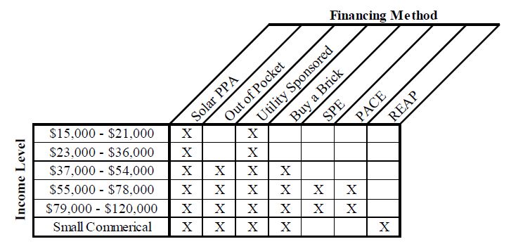
Although the costs of residential or small business PV systems can be a factor that pushes prospective clients away, initiatives set forth by local and federal governments are driving these costs down. For example, the Department of Energy’s (DOE) Solar Sunshot Initiative have been supporting the research, design, and implementation of low-cost, high efficiency PV technologies in order to make solar electricity cost-competitive with other sources by 2020 [1]. Even with the DOE’s aggressive approach, the cost of a PV system can still be a burden on many prospective owners. The median installed price was $4.3/W for residential systems in 2014 [5]; thus the cost of a system becomes a large investment for most systems. SunShot’s objective is to have the cost of residential systems down to $1.50/W by the year 2020 [6]. To help alleviate this burden, new and unique payment plans are being designed to accommodate individuals depending on various factors including their income levels. Solar Powering Your Community: A Guide for Local Governments [7] provides a list of funding options that an individual or an entire community can investigate in order to mitigate the costs. With prices of PV technology expected to decrease in future years, expected payback periods should also decrease, resulting in an overall shorter payback period for PV systems. In 2007 the Department of Energy chose the Northeast Denver Housing Center (NDHC) as a pilot program for the Solar America Showcase program. The intent of this pilot program was to set up a model for the creation of a new residential finance model for the installation of PV systems in low-income residential areas. The program had to incorporate a low-income training program for residents in that area, an energy conservation incentive program, and a program for integration of renewable energy systems onto existing affordable housing developments [8]. The housing units that received systems were very low-income families who generally earned less than 60% of the median income ($36,480). In order to afford this program the NDHC established a power purchase agreement with a third-party investor with funds received from Colorado’s Governor’s Energy Office. The NDHC will purchase power from the third-party for a 20 year term in which they will pay $.08/kWh for the first year, and then prices will escalate at a rate of 5% per year for the term of the agreement [8]. In order to pay for the systems installed in the low-income areas, the NDHC charged tenants an increase of $25 per month on their electricity bill; however, the tenants will receive a decreased utility cost to cover the natural gas portion of their monthly energy expenses. Another stipulation of the pilot program included job training and tenant education for the low-income residents. This type of renewable energy financing programs drives the price of a PV system down, which can make it affordable for residential and commercial clients alike. The payment options presented in this paper are ones that are currently available to customers in Illinois. Recommendations for options available outside of Illinois will be presented in the discussion section. Payments options currently available include the following and they are summarized in Table 1
| Funding and Payment Options (PPA) | Financing Schemes |
| Power Purchase Agreement | · A third-party developer owns, operates, and maintains |
| · A host customer agrees to site the system on their property | |
| · Allows the customer to buy electricity at a set cost for a given with no upfront cost | |
| Community Solar | · Provides electricity to a defined community but the system itself does not have to be directly on rooftops |
| · Increase the access to solar for whom cannot install solar on their property such as a residence in shaded areas, rental properties, and multi-unit housing | |
| Out-of-pocket Purchase | · Property owner responsible for financing the system |
| · Benefits include financial gains through renewable energy credits, investment returns, and insurance against increased electricity rates | |
| Property Assessed Clean Energy Financing (PACE) | · A finance method to address the upfront cost |
| · Provides a long-term fixed cost financing option, a repayment obligation that can transfer, and federal tax benefits | |
| Rural Energy for American Program (REAP) | · Financial assistance to agricultural producers and to small businesses in rural America |
| · Provides guaranteed loans and grants |
 DownLoad: CSV
A power purchase agreement (PPA) is a financial agreement in which a third-party developer owns, operates, and maintains the PV system, and a host customer agrees to site the system on their roof or elsewhere on their property, and also agrees to purchase the PV systems electric output for a predetermined period [9]. The main benefit of a PPA is that it allows the customer to buy electricity at a set cost a given number of years, which provides insurance against fluctuating energy prices during those years. Another main benefit is that there is no upfront cost for the customer. The third-party provides all funding for the system and is responsible for any maintenance issues during the duration of their agreement. Once the agreement is over, the customer and third-party have the option to renew the agreement, the customer can purchase the system at its value, or the third party must remove the system from the customer’s property. This option is suitable for any income level, however it is especially appropriate for lower income levels, as no upfront cost is required.
Community solar, also called shared solar is defined as a solar PV system that, through a defined voluntary program, provides power and/or financial benefits [10]. A major benefit for community-owned solar is that it provides electricity to a defined community, but the system itself does not have to be directly on the rooftops of the residences within that community. In fact, a study by NREL in 2008 found that only 22 to 27% of residential rooftop areas are suitable for hosting an on-site PV system [10]. NREL has provided three alternative models for community solar as listed below:
• Utility Sponsored Systems, in which a utility owns and operates the system that is open to voluntary ratepayer participation.
• Buy a Brick wherein community members contribute to a community owned installation, and are allocated a percent of the electricity that is generated.
• Special Purpose Entity model (SPE) in which individual investors join a business enterprise to develop a community solar project.
One major benefit to community solar is that it can increase the access to solar electricity for those members who cannot install solar on their property. This would include a residence in shaded areas, where rooftop or ground mount systems are not suitable; it would also include rental properties and multi-unit housing where residents are not the owner of the property. There are at least 31 shared/community owned renewable projects in 12 different states throughout the U.S [11].
In the case of an out-of-pocket purchase, homeowners and business owners would be responsible for the entire payment of the PV system. Benefits of this option include sole ownership of the system. Benefits would additionally include any financial gains that the system may bring in such as Solar Renewable Energy Credits, investment returns once the system is paid off, and insurance against increased electricity rates in the future. However, since the owners are responsible for the system, they must pay for any maintenance or system problems costs. In some states the use of a direct incentive or production-based incentive such as a cash rebate has been used to lower the cost of the system for out-of-pocket purchases. These grants and rebates are often based on solar system capacity or system cost [12]. Along with 23 other states, Illinois is one of the states that have direct cash incentives for PV systems [12].
The PACE program is a finance method used for renewable energy and energy-efficient investments; it is meant to address both the upfront cost barriers to solar and the hesitancy of homeowners to make long-term investments in their homes [12]. The way the PACE program works is that the city or county finances the upfront cost of the energy investment, either directly or intermittently for the private investors. The property owner then repays the loan over an extended period through a special property tax assessment. The main benefits of the PACE program are it provides a long-term fixed cost financing option, a repayment obligation that can transfer with the sale of the property, and the potential to deduct the loan interest from federal taxable income as part of a local property tax deduction. An example is in Boulder, Colorado, where PACE provided $40 million in bonds to offer special financing options for renewable energy and energy-efficient improvements to local residents. The loan to each resident is repaid over 15 years, and the key requirement of the agreement is that applicants must attend a workshop to learn about the program requirements and to receive information on the benefits of investing in energy efficiency measures [12]. Illinois has enacted PACE enabling legislation, and there is growing interest in developing programs for customers [13].
Similar to PACE, REAP is a program that provides financial assistance to agricultural producers and to small businesses in rural America to purchase, install, and construct renewable energy systems [14]. REAP provides guaranteed loans and grants to assist qualified applicants. With this type of loan, small businesses within the designated boundary would be qualified for the grants and loans, which would cover up to 75% of the total eligibleproject costs; and then the Renewable Energy System Grant could additionally cover up to 25% of the eligible cost.
The Solar Foundation reports that as of a November 2014, there were 173,807 solar jobs in the United States [15], an increase of roughly 31,000 positions from previous year. Solar jobs are defined as workers who spend at least 50% of their time supporting solar-related activities. The Solar Foundation predicts positive industry growth for the next 12 months; specifically, it predicts a growth of 21.8% during that time period, compared to the overall economy, which is expected to grow at a rate of 1.1%. For those categorized as solar workers, the median average salary for installer was between $20-24 per hour, making it competitive with pay for related positions that require work experience; however no advanced educational degree is needed. Croucher [16] performed an economic impact study of installing solar PV Systems in each of the U.S. states. Using the same modeling software (National Renewable Energy Laboratory’s (NREL) Jobs and Economic Development Impact (JEDI)) as this present study, software from the he determined which state derives the greatest statewide economic impact for a given amount of solar deployment [16]. JEDI is an input-output modeling software that measures the spending patterns and location- specific economic structures to reflect expenditures supporting varying levels of employment, income, and output [17]. For his model, Croucher kept all inputs at their default selection in order to create equal ground for the study. The model for each state was the installation of 100 2.5 kW PV systems for new residential construction. His results found that out of all 50 states, Pennsylvania lead the way in terms of jobs created totaling 28.98 jobs per 100 systems. Illinois maintained second place by creating 27.65 jobs per 100 systems. A study, released in October of 2013, conducted by the Solar Foundation titled An Assessment of the Economic Revenue and Societal Impacts of Colorado’s Solar Industry, presented a snapshot of the economic and social impacts of the industry within Colorado [18]. The Foundation obtained its data from GTM Research/Solar Energy Industries Association’s U.S. Solar Market Insight from 2007-2013. This data was used for inputs into the JEDI software to find jobs created to date as well as revenues produced, earnings, andenvironmental impacts of PV installations. The Solar Foundation also conducted a scenario analysis using JEDI to predict impacts of Colorado’s Million Dollar Roof campaign. According to this study, since the year 2007, more than 10,000 jobs have been created while total earnings have accumulated $546 M. Loomis et al. [17] determined the job creation that would occur if the state installed more large-scale utility photovoltaic systems. By using results from a previous study they had conducted [19], they were able to determine what type of impact utility scale PV installations would have on the statewide economy in terms of job creation in Illinois. Different scenarios were used, thus deriving different outputs in terms of job creation. Each scenario included direct, indirect, and induced impacts, which are three distinct economic impacts. Out of this process, nine models were created with employment predictions ranging from 26,812 to 131,779 jobs statewide [17].
In order to adequately conduct an economic impact study for the Town of Normal, we utilized the economic and social characteristics that define Normal. A set of data was gathered on the income levels from the year 2012 [23]. Subsequently we overlaid the income level data collected on geographic information systems (GIS), which allows the towns’ income levels to be presented on the map of the town. We then subdivided the town based upon different income levels.
The town has a wide variation in terms of housing characteristics. Again, the Census Bureau data were used to find the Town of Normal’s housing breakdown. We have obtained information regarding housing units, the built year, the total number of rooms within the housing unit, housing tenure, average household size, year the household was occupied, and the different types of fuel used. These characteristics are beneficial when deciding which type of payment option is ideal for the different areas of the case study area. For the PV system size appropriate for each building unit, the outcomes of the first phase of this research study [20] were utilized to assess the jobs and economic impacts due to PV system implementation.
For jobs and economic development impacts analysis, we utilized the Jobs and Economic Development Impacts (JEDI) Model. These models were developed by Marshall Goldberg of MRG & Associates, under contract with the National Renewable Energy Laboratory. The JEDI model utilizes multipliers obtained from IMPLAN which is maintained by the Minnesota IMPLAN Group, Inc. For the purposes of this study, the state-level multipliers built into JEDI were replaced with county-level multipliers for McLean County purchased from the Minnesota IMPLAN Group, Inc [21].
Economic multipliers are derived from industry input-output tables that detail the interrelationships between different sectors of the economy. Multipliers show how an additional dollar of spending in one sector of the economy will ripple through the economy by spurring spending in other sectors to provide that inputs into that sector. Because of differences in the economy across different geographies, economic multipliers vary depending on specific industries located in the area being studied. If an input is not sourced local, that is treated as a “leakage” from the economic impact to that specific territory.
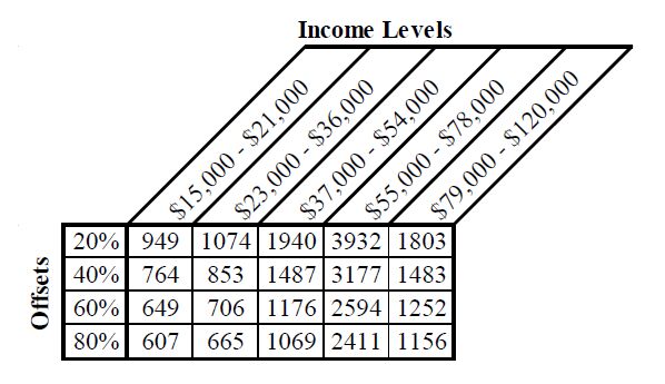
Given that each income level is comprised of different characteristics when it comes to available funds to spend on a PV system, we created a matrix to show possible payment options at the various levels. The authors’ previous study [20] conducted a detailed analysis to identify the rooftops in the Town of Normal, Illinois that are best suited for distributed generation solar photovoltaic applications, to quantify their energy generation potential, and to evaluate the subsequent carbon mitigation potential. Percentage offsets represent the capacity of each system to reduce electrical demand depending on the average electrical consumption of the buildings in the case study area. Based upon the outcomes of this study and the literature review on a variety of financing schemes, feasible financing options were suggested to each income class. Small commercial and residential buildings that were included in the study were south facing or flat roofs only. The GIS analysis conducted in [20] revealed which buildings were applicable for each sized system as shown in Table 2.
| Percentage Offset | System Size | Number of Systems |
| 20% | 1.5 kW | 9,698 |
| 40% | 3 kW | 7,764 |
| 60% | 4.5 kW | 6,333 |
| 80% | 5.3 kW | 5,908 |
DownLoad: CSVThe economic analysis of PV development presented here uses the NREL’s latest Jobs and Economic Development Impacts (JEDI) PV Model (PV10.17.11). The JEDI PV Model is an input-output model that measures the spending patterns and location-specific economic structures that reflect expenditures supporting varying levels of employment, income, and output for solar PV [22]. That is, the JEDI Model takes into account that the output of one industry can be used as an input for another. For example, when a PV system is installed, there are both soft costs consisting of permitting, installation and customer acquisition costs, and hardware costs, of which the PV module is the largest component. The purchase of a module not only increases demand for manufactured components and raw materials, but also supports labor [17]. When an installer and/or developer purchases a module from a manufacturing facility, the manufacturer uses some of that money to pay employees. The employees use a portion of their compensation to purchase goods and services within their community.
The total economic impact can be broken down into three distinct types including direct impacts, indirect impacts, and induced impacts [22]. Direct impacts during the construction period refer to the changes that occur in industries directly hired to install the PV system. Indirect impacts during construction period consist of the changes in inter-industry purchasesresulting from the supply chain impacts of purchases of parts that make up the PV system and associated parts [17]. Induced impacts during construction refer to the changes that occur in household spending as household income increases due to increased construction of PV systems [17].
Table 3 represents which payment options are best suited for each income level. The lower the income level the fewer options are available. Income levelsranging from $15,000 to $36,000 were best suited for either a PPA or a Utility Sponsored program. Based off of the Massachusetts Institute of Technologies’ wage calculator [23], $37,000-$54,000 is the yearly income at which residents exceed their living wage. Discretionary income, or excess income, could now be allocated for items such as a PV system. Small commercial buildings were additionally provided the option of using REAP, which is available only to rural business or agricultural institutions.
Table 4 breaks down how many systems can be installed given the income level and the percentage being offset. Higher income levels were able to support larger systems while the lower income levels, which generally had small roof areas, were only able to support of fraction of systems.
 |
DownLoad: CSVUsing the JEDI model, we assess the economic impact of the four solar scenarios that were developed from the companion analysis. Depending on how technical potential is measured, we estimate the economic impact for four levels of demand—20%, 40%, 60% and 80%. A key driver of the economic impact of these different demand levels is how much of the labor and materials are sourced from within McLean County. We assume throughout the study that the solar panels are not manufactured within McLean County since there is no local manufacturer currently and we do not expect a new manufacturer to locate here. To show the possible jobs impact of growing the local solar system materials and services locally, we run two different assumptions. First, we assume the JEDI defaults. Second, we assume all of the services are sourced locally (except solar panels). Thus, we perform 8 different model runs as shown in Table 5 below:
| Technical PotentialSourced | within McLean County | |
| Default | 100% (excluding panels) | |
| 20% | Model 1 | Model 2 |
| 40% | Model 3 | Model 4 |
| 60% | Model 5 | Model 6 |
| 80% | Model 7 | Model 8 |
DownLoad: CSVIn addition to the technical potential and percentage manufactured in McLean County, there are several assumptions built into the model that do not changebetween the model runs. The default settings within JEDI assume 100 residential retrofit fixed-mount crystalline-silicon systems having a nameplate capacity of 5 kW. The installed system cost is $6,562 and the annual direct operations and maintenance expense is $32.80. We do not vary the installed system cost or the operations and maintenance expense between model runs. Table 6 shows the jobs impacts for the eight different scenarios that were run for the construction phase of the projects. The jobs are reported in job-years and based on full time equivalents. This type of measurement of the jobs impacts enables us to do an apples-to-apples comparison. By this measurement, one full-time construction job lasting for one year is equivalent to 2 full-time jobs lasting six months or 4 full-time jobs lasting three months. As shown in Table 6, the total employment impacts vary from 377.4 to 1059.5 job years.
| Percentage Manufactured in McLean County | ||
| Technical Potential | Default | 100% |
| 20% | 377.4 | 492.2 |
| 40% | 604.2 | 788.1 |
| 60% | 739.3 | 964.3 |
| 80% | 812.2 | 1,059.50 |
DownLoad: CSVTable 7 shows the ongoing operations and maintenance jobs that will result under each scenario. The operations and maintenance jobs are not dependent on where the original equipment was manufactured, so the jobs impact only varies by the assumed installed capacity. Although some replacement parts will be required from time to time, the supply chain impacts from this small amount of equipment is overshadowed by the direct labor involved in operations and maintenance. The employment impacts during the operating years vary from 18.8 to 40.5. Because there are few existing solar installations in McLean County and the industry is not well developed, all of the labor would be sourced from outside the County under the Default scenarios using existing economic multipliers.
| Technical Potential | Default | 100% |
| 20% | 0 | 18.8 |
| 40% | 0 | 30.1 |
| 60% | 0 | 36.8 |
| 80% | 0 | 40.5 |
DownLoad: CSVWhen measuring the economic impact, one is concerned with the earnings of these workers as well as the total number of jobs created. Table 8 shows the total McLean County earnings impacts for the eight different scenarios that were run for the construction phase. The earnings are reported in thousands of 2012 dollars so that they are adjusted for the fact that jobs created in future years may have higher earnings due to inflation alone. As shown in Table 8, the total earnings impacts vary from $30.3 million to $65.2 million.
| Technical Potential | Default | 100% |
| 20% | $23,282.60 | $30,300.80 |
| 40% | $37,279.10 | $48,516.20 |
| 60% | $45,612.10 | $59,361.10 |
| 80% | $50,115.80 | $65,222.40 |
DownLoad: CSVThe final and largest measure of economic impact is total output impacts. Table 9 shows the total McLean County output impacts for the eight different scenarios that were run for the construction phase. Output is reported in thousands of 2012 dollars so that they are adjusted for the fact that output in future years may be higher due to inflation alone. As shown in Table 9, the total earnings impacts vary from $68.5 million to $165.6 million.
| Technical Potential | Percentage Manufactured in McLean County | |
| Default | 100% | |
| 20% | $68,531.40 | $76,932.90 |
| 40% | $109,729.30 | $123,181.60 |
| 60% | $134,257.30 | $150,716.50 |
| 80% | $147,513.70 | $165,598.10 |
DownLoad: CSVThis study has created a simplified model for both the purchasing process as well as the selling and designing process that is attached to the acquisition of soft and hard goods related to solar products. As each percentage option has a fixed nameplate capacity, as well as a fixed price, the burden on the PV providers of designing specific systems for each building is eliminated. Any potential customer could specify which percent system they wished to have installed, and the solar installer would know the exact specifications required.
A possible funding solution for distributed systems would be to institute a feed-in tariff (FIT). Feed-in tariffs require energy suppliers to buy electricity produced from renewable resources at a fixed price per kilowatt-hour, usually for a fixed period [8]. FITs are seen globally and are accepted as the main driver for renewable technology implementation. State and local governments can implement such a tariff by incorporating it into their renewable portfolio standard (RPS). Along with their RPS, FITs can advance the development process of renewable technologies throughout the country. Future research could look at all possible payment methods used in the country and throughout the world.
This study used available funding options for PV in the state of Illinois to provide payment options to residents in the Town of Normal, IL. Given information collected from literature reviews and case studies, the payment options were suggested viable methods for residential and small commercial buildings given their income levels. An economic impact study was conducted in order to quantify job creation due to PV installations at eachpercent level. The estimated stimulus respective to each level of implementation can potentially impact a broad spectrum of income levels. This research study’s objective of deployment optimization required a thorough analysis and proper consideration, given the prospect of positive implications on those who participate in Normal, Illinois.
The authors declare no conflicts of interest regarding this paper.
| [1] | Flegal KM, Carroll MD, Ogden CL, et al. (2010) Prevalence and trends in obesity among US adults, 1999-2008. JAMA 303(3): 235-241. |
| [2] | Ogden CL, Carroll MD, Curtin LR, et al. (2010) Prevalence of high body mass index in US children and adolescents, 2007-2008. JAMA 303(3): 242-249. |
| [3] | Flegal KM, Carroll MD, Kit BK, et al. (2012) Prevalence of obesity and trends in the distribution of body mass index among US adults, 1999-2010. JAMA 307(5): 491-497. |
| [4] | Ogden CL, Carroll MD, Kit BK, et al. (2012) Prevalence of obesity and trends in body mass index among US children and adolescents, 1999-2010. JAMA 307(5): 483-490. |
| [5] | Mei Z, Scanlon KS, Grummer-Strawn LM, et al. (1998) Increasing prevalence of overweight among US low-income preschool children: the Centers for Disease Control and Prevention pediatric nutrition surveillance, 1983 to 1995. Pediatr 101(1): E12. |
| [6] | Mokdad AH, Serdula MK, Dietz WH, et al. (2000) The continuing epidemic of obesity in the United States. JAMA 284(13): 1650-1651. |
| [7] | Webber LS, Cresanta JL, Croft JB, et al. (1986) Transitions of cardiovascular risk from adolescence to young adulthood—the Bogalusa Heart Study: II. Alterations in anthropometric blood pressure and serum lipoprotein variables. J Chron Dis 39(2): 91-103. |
| [8] | Serdula MK, Ivery D, Coates RJ, et al. (1993) Do obese children become obese adults? A review of the literature. Prev Med 22(2): 167-177. |
| [9] | Guo SS, Roche AF, Chumlea WC, et al. (1994) The predictive value of childhood body mass index values for overweight at age 35 y. Am J Clin Nutr 59(4): 810-819. |
| [10] | Calle EE, Rodriguez C, Walker-Thurmond K, et al. (2003) Overweight, obesity, and mortality from cancer in a prospectively studied cohort of U. S. adults. N Engl J Med 348(17): 1625-1638. |
| [11] | Shike M. (1996) Body weight and colon cancer. Am J Clin Nutr 63(3 Suppl): 442S-444S. |
| [12] | Murphy TK, Calle EE, Rodriguez C, et al. (2000) Body mass index and colon cancer mortality in a large prospective study. Am J Epidemiol 152(9): 847-854. |
| [13] | Bungum T, Satterwhite M, Jackson AW, et al. (2003) The relationship of body mass index, medical costs, and job absenteeism. Am J Health Behav 27(4): 456-462. |
| [14] | Fontaine KR, Redden DT, Wang C, et al. (2003) Years of life lost due to obesity. JAMA 289(2):187-193. |
| [15] | Ford ES, Moriarty DG, Zack MM, et al. (2001) Self-reported body mass index and health-related quality of life: findings from the Behavioral Risk Factor Surveillance System. Obes Res 9(1):21-31. |
| [16] | Sturm R, Ringel JS, Andreyeva T. (2004) Increasing obesity rates and disability trends. Health Aff (Millwood) 23(2): 199-205. |
| [17] | Burton WN, Chen CY, Schultz AB, et al. (1999) The costs of body mass index levels in an employed population. Stat Bull Metrop Insur Co. 80(3): 8-14. |
| [18] | Cawley J, Meyerhoefer C. (2012) The medical care cost of obesity: an instrumental variables approach. J Health Econ 31(1): 219-230. |
| [19] | Wojcicki JM, Heyman MB. (2012) Reducing childhood obesity by eliminating 100% fruit juice. Am J Public Health 102(9): 1630-1633. |
| [20] | Santos FL, Esteves SS, da Costa Pereira A, et al. (2012) Systematic review and meta-analysis of clinical trials of the effects of low carbohydrate diets on cardiovascular risk factors. Obes Rev 13(11): 1048-1066. |
| [21] | Wycherley TP, Moran LJ, Clifton PM, et al. (2012) Effects of energy-restricted high-protein, low-fat compared with standard-protein, low-fat diets: a meta-analysis of randomized controlled trials. Am J Clin Nutr 96(6): 1281-1298. |
| [22] | 25. Lustig R. Fat Chance. (2012) Beating the odds against sugar, processed food, obesity, and disease. New York: Hudson Street Press. |
| [23] | 26. Medical College of Wisconsin. Elimination of Juice/Empty Calories. (2013) Available from: http://www. mcw. edu/NDTN/Overweight/DietInterventions/EliminationofJuiceEmptyCalories. ht m. (Accessed on April 26, |
| [24] | 27. O'Neil C, Nicklas T. (2008) A Review of the Relationship between 100% Fruit Juice Consumption and Weight in Children and Adolescents. Am J Lifestyle Med 2(4): 315-354. |
| [25] | 28. Dharmasena S, Capps O, Jr. (2012) Intended and unintended consequences of a proposed national tax on sugar-sweetened beverages to combat the U. S. obesity problem. Health economics 21(6): 669-694. |
| [26] | 29. Fletcher JM, Frisvold DE, Tefft N. (2011) Are soft drink taxes an effective mechanism for reducing obesity? J Policy Anal Manage 30(3): 655-662. |
| [27] | 33. Bray GA. (2013) Energy and fructose from beverages sweetened with sugar or high-fructose corn syrup pose a health risk for some people. Adv Nutr 4(2): 220-225. |
| [28] | 34. Lustig R. (2013) Fructose: It's "Alcohol without the Buzz". Adv Nutr 4(2): 226-235. |
| [29] | 35. Rippe J, Angelopoulos T. (2013) Sucrose, high-fructose corn syrup, and fructose, their metabolism and potential health effects: what do we really know? Adv Nutr 4(2): 236-245. |
| [30] | 36. White J. (2013) Challenging the fructose hypothesis: New perspectives on fructose consumption and metabolism. Adv Nutr 4(2): 246-256. |
| [31] | 37. Klurfeld D. (2013) What do government agencies consider in the debate over added sugars? Adv Nutr 4(2): 257-261. |
| [32] | 38. Gillespie D. (2008) Sweet poison: Why sugar is making us fat. Melbourne: Viking Australia. |
| [33] | 39. Max Rubner——1854-1932. (1965) Energy physiologist. JAMA 194(1): 86-87. |
| [34] | 40. von Noorden C. (2013) Clinical Treatises on the Pathology and Therapy of Disorders (Vol. 1). Charleston: Nabu Press. |
| [35] | 41. Sievenpiper J, de Souza R, Mirrahimi A, et al. (2012) Effect of fructose on body weight in controlled feeding trials: a systematic review and meta-analysis. Ann Intern Med 156(4):291-304. |
| [36] | 42. Ha V, Sievenpiper JL, de Souza RJ, et al. (2012) Effect of fructose on blood pressure: a systematic review and meta-analysis of controlled feeding trials. Hypertension 59(4): 787-795. |
| [37] | 43. Sievenpiper JL, Carleton AJ, Chatha S, et al. (2009) Heterogeneous effects of fructose on blood lipids in individuals with type 2 diabetes: systematic review and meta-analysis of experimental trials in humans. Diabetes Care 32(10): 1930-19 |
| [38] | 44. Cozma AI, Sievenpiper JL, de Souza RJ, et al. (2012) Effect of fructose on glycemic control in diabetes: a systematic review and meta-analysis of controlled feeding trials. Diabetes Care 35(7):1611-1620. |
| [39] | 45. Sievenpiper JL, Chiavaroli L, de Souza RJ, et al. (2012) 'Catalytic' doses of fructose may benefit glycaemic control without harming cardiometabolic risk factors: a small meta-analysis of randomised controlled feeding trials. Br J Nutr 108(3): 418-423. |
| [40] | 49. Krebs-Smith SM, Guenther PM, Subar AF, et al. (2010) Americans do not meet federal dietary recommendations. J Nutr 110): 1832-1838. |
| [41] | 50. Freeland-Graves J, Nitzke S. (2013) Position of the Academy of Nutrition and Dietetics: Total diet approach to healthy eating. J Acad Nutr Diet 113(2): 307-317. |
| [42] | 53. Nitzke S, Freeland-Graves J. (2007) Position of the American Dietetic Association: Total diet approach to communicating food and nutrition information. J Am Diet Assoc 107: 7. |
| [43] | 54. Briefel RR, Wilson A, Cabili C, et al. (2013) Reducing calories and added sugars by improving children's beverage choices. J Acad Nutr Diet 113(2): 269-275. |
| [44] | 55. Barclay AW, Brand-Miller J. (2011) The Australian paradox: a substantial decline in sugars intake over the same timeframe that overweight and obesity have increased. Nutrients 3(4):491-504. |
| [45] | 56. Welch J, Sharma A, Grellinger L, et al. (2011) Consumption of added sugars is decreasing in the United States. Am J Clin Nutr 94(3): 726-734. |
| [46] |
57. Sylvetsky A, Welsh J, Brown R, et al. (2012) Low-calorie sweetener consumption is increasing in the United States. Am J Clin Nutr 96: 640-6 doi: 10.3945/ajcn.112.034751

|
| [47] | 59. Ford E, Dietz W. (2013) Trends in energy intake among adults in the United States: findings from NHANES. Am J Clin Nutr 97(4): 848-853. |
| [48] | 60. Malik VS, Schulze MB, Hu FB. (2006) Intake of sugar-sweetened beverages and weight gain: a systematic review. Am J Clin Nutr 84(2): 274-288. |
| [49] | 61. Vartanian LR, Schwartz MB, Brownell KD. (2007) Effects of soft drink consumption on nutrition and health: a systematic review and meta-analysis. Am J Public Health 97(4): 667-675. |
| [50] | 62. Olsen NJ, Heitmann BL. (2009) Intake of calorically sweetened beverages and obesity. Obes Rev10(1): 68-75. |
| [51] | 63. Wolff E, Dansinger ML. (2008) Soft drinks and weight gain: how strong is the link? Medscape J Med 10(8): 189. |
| [52] | 64. Malik VS, Popkin BM, Bray GA, et al. (2010) Sugar-sweetened beverages, obesity, type 2 diabetes mellitus, and cardiovascular disease risk. Circulation 121(11): 1356-1364. |
| [53] | 65. van Dam R, Seidell J. (2007) Carbohydrate intake and obesity. Europ J Clin Nutr 61(Suppl 1):S75-S99. |
| [54] | 66. Woodward-Lopez G, Kao J, Ritchie L. (2010) To what extent have sweetened beverages contributed to the obesity epidemic? Public Health Nutr 14(3): 499-509. |
| [55] |
67. Te Morenga l, Mallard S, Mann J. (2012) Dietary sugars and body weight: systematic review and meta-analyses of randomised controlled trials and cohort studies. Br Med J 346: e7492. doi: 10.1136/bmj.e7492
|
| [56] | 68. Pereira MA, Jacobs DR, Jr. (2008) Sugar-sweetened beverages, weight gain and nutritional epidemiological study design. Br J Nutr 99(6): 1169-1170. |
| [57] | 69. Bachman CM, Baranowski T, Nicklas TA. (2006) Is there an association between sweetened beverages and adiposity? Nutr Rev 64(4): 153-174. |
| [58] | 70. Gibson S. (2008) Sugar-sweetened soft drinks and obesity: a systematic review of the evidence from observational studies and interventions. Nutr Res Rev 21(2): 134-147. |
| [59] | 71. Mattes RD, Shikany JM, Kaiser KA, et al. (2011) Nutritively sweetened beverage consumption and body weight: a systematic review and meta-analysis of randomized experiments. Obes Rev12(5): 346-365. |
| [60] | 72. Libuda L, Kersting M. (2006) Soft drinks and body weight development in childhood: is there a relationship? Curr Opin Clin Nutr Metab Care 12(6): 596-. |
| [61] | 73. Van Baak M, Astrup A. (2009) Consumption of sugars and body weight. Obes Rev 10(Suppl 1):9-23. |
| [62] |
74. Monasta L, Batty G, Cattaneo A, et al. (2010) Early-life determinanats of overweight and obesity: a review of systematic reviews. Obes Rev 11: 695-708. doi: 10.1111/j.1467-789X.2010.00735.x
|
| [63] | 75. Forshee RA, Anderson PA, Storey ML. (2008) Sugar-sweetened beverages and body mass index in children and adolescents: a meta-analysis. Am J Clin Nutr 87(6): 1662-1671. |
| [64] | 76. Ruxton CH, Gardner EJ, McNulty HM. (2010) Is sugar consumption detrimental to health? A review of the evidence 1995-2006. |
| [65] | 77. Janssen I, Katmarzyk PT, Boyce WF, et al. (2005) Health behaviour in school-aged children obesity working group: Comparison of overweight and obesity prevalence in school-aged youth from 34 countries and their relationships with physical activity and dietary patterns. Obes Rev6(2): 123-132. |
| [66] | 78. Weed DL, Althuis MD, Mink PJ. (2011) Quality of reviews on sugar-sweetened beverages and health outcomes: a systematic review. Am J Clin Nutr 94(5): 1340-1347. |
| [67] | 79. Cope MB, Allison DB. (2010) White hat bias: examples of its presence in obesity research and a call for renewed commitment to faithfulness in research reporting. Int J Obes (Lond) 34(1):84-88. |
| [68] | 80. James J, Thomas P, Cavan D, et al. (2004) Preventing childhood obesity by reducing consumption of carbonated drinks: cluster randomised controlled trial. Br Med J 328(7450):1237. |
| [69] | 81. Ebbeling CB, Feldman HA, Osganian SK, et al. (2006) Effects of decreasing sugar-sweetened beverage consumption on body weight in adolescents: a randomized, controlled pilot study. Pediatrics 117(3): 673-680. |
| [70] | 82. Nicklas T, O'Neil C, Liu Y. (2011) Intake of added sugars is not associated with weight measures in children 6-18 years of age: NHANES 2003-2006. Nutr Res 31(5): 338-346. |
| [71] | 83. Storey ML, Forshee RA, Weaver AR, et al. (2003) Demographic and lifestyle factors associated with body mass index among children and adolescents. Int J Food Sci Nutr 54(6): 491-503. |
| [72] | 84. Marriott BP, Olsho L, Hadden L, et al. (2010) Intake of added sugars and selected nutrients in the United States, National Health and Nutrition Examination Survey (NHANES) 2003-2006. Crit Rev Food Sci Nutr 50(3): 228-258. |
| [73] | 85. Fisher JO, Mitchell DC, Smiciklas-Wright H, et al. (2001) Maternal milk consumption predicts the tradeoff between milk and soft drinks in young girls' diets. J Nutr 131(2): 246-250. |
| [74] | 86. Harnack L, Stang J, Story M. (1999) Soft drink consumption among US children and adolescents: nutritional consequences. J Am Diet Assoc 99(4): 436-441. |
| [75] | 87. Anderson GH, Luhovyy B, Akhavan T, et al. (2011) Milk proteins in the regulation of body weight, satiety, food intake and glycemia. Nestle Nutr Workshop Ser Pediatr Program 67:147-159. |
| [76] | 88. Barba G, Russo P. (2006) Dairy foods, dietary calcium and obesity: a short review of the evidence. Nutr Metab Cardiovasc Dis 16(6): 445-451. |
| [77] | 89. Deddo L. (2007) Connecting the dots. Aeon Publishing Inc. Available from: http://www. amazon. com/Connecting-The-Dots-Leonard-Deddo/dp/1595266941/ref=sr_1_1?ie= UTF8&qid=1364933001&sr=8-1&keywords=Connecting+the+Dots+leonard+deddo. (Accessed on April 2, 2013). |
| [78] | 90. Darmon N, Drewnowski A. (2008) Does social class predict diet quality? Am J Clin Nutr 87(5):1107-1117. |
| [79] | 91. Monsivais P, Drewnowski A. (2009) Lower-energy-density diets are associated with higher monetary costs per kilocalorie and are consumed by women of higher socioeconomic status. J Am Diet Assoc 109(5): 814-822. |
| [80] | 92. Brownell KD, Farley T, Willett WC, et al. (2009) The public health and economic benefits of taxing sugar-sweetened beverages. N Engl J Med 361(16): 1599-1605. |
| [81] | 93. Brownell KD, Frieden TR. (2009) Ounces of prevention—the public policy case for taxes on sugared beverages. N Engl J Med 360(18): 1805-1808. |
| [82] | 94. Fletcher J, Frisvold D, Tefft N. (2010) Can soft drink taxes reduce population weight? Contemp Econ Policy 28(1): 23-35. |
| [83] | 96. Fletcher JM, Frisvold DE, Tefft N. (2010) The effects of soft drink taxes on child and adolescent consumption and weight outcomes. J Public Econ 94(11-12): 967-974. |
| [84] | 97. Sturm R, Powell LM, Chriqui JF, et al. Deddo L. (2010) Soda Taxes, Soft Drink Consumption, And Children's Body Mass Index. Health Affairs 29(5): 1052-1058. |
| [85] | 98. Ogden CL, Kit BK, Carroll MD, et al. (2011) Consumption of sugar drinks in the United States, 2005-2008. NCHS Data Brief 71: 1-8. |
| [86] | 99. Cohen DA, Sturm R, Scott M, et al. Deddo L. (2010) Not Enough Fruit and Vegetables or Too Many Cookies, Candies, Salty Snacks, and Soft Drinks? Public Health Rep 125: 88-95. |
| [87] | 100. Reedy J, Krebs-Smith SM. Deddo L. (2010) Dietary sources of energy, solid fats, and added sugars among children and adolescents in the United States. J Am Diet Assoc 110(10):1477-1484. |

Figures(2)

Theresa A. Nicklas, Carol E. O'Neil. Prevalence of Obesity: A Public Health Problem Poorly Understood[J]. AIMS Public Health, 2014, 1(2): 109-122. doi: 10.3934/publichealth.2014.2.109

| Funding and Payment Options (PPA) | Financing Schemes |
| Power Purchase Agreement | · A third-party developer owns, operates, and maintains |
| · A host customer agrees to site the system on their property | |
| · Allows the customer to buy electricity at a set cost for a given with no upfront cost | |
| Community Solar | · Provides electricity to a defined community but the system itself does not have to be directly on rooftops |
| · Increase the access to solar for whom cannot install solar on their property such as a residence in shaded areas, rental properties, and multi-unit housing | |
| Out-of-pocket Purchase | · Property owner responsible for financing the system |
| · Benefits include financial gains through renewable energy credits, investment returns, and insurance against increased electricity rates | |
| Property Assessed Clean Energy Financing (PACE) | · A finance method to address the upfront cost |
| · Provides a long-term fixed cost financing option, a repayment obligation that can transfer, and federal tax benefits | |
| Rural Energy for American Program (REAP) | · Financial assistance to agricultural producers and to small businesses in rural America |
| · Provides guaranteed loans and grants |
DownLoad: CSV |
DownLoad: CSV| Technical PotentialSourced | within McLean County | |
| Default | 100% (excluding panels) | |
| 20% | Model 1 | Model 2 |
| 40% | Model 3 | Model 4 |
| 60% | Model 5 | Model 6 |
| 80% | Model 7 | Model 8 |
DownLoad: CSV| Percentage Manufactured in McLean County | ||
| Technical Potential | Default | 100% |
| 20% | 377.4 | 492.2 |
| 40% | 604.2 | 788.1 |
| 60% | 739.3 | 964.3 |
| 80% | 812.2 | 1,059.50 |
DownLoad: CSV| Technical Potential | Default | 100% |
| 20% | 0 | 18.8 |
| 40% | 0 | 30.1 |
| 60% | 0 | 36.8 |
| 80% | 0 | 40.5 |
DownLoad: CSV| Technical Potential | Default | 100% |
| 20% | $23,282.60 | $30,300.80 |
| 40% | $37,279.10 | $48,516.20 |
| 60% | $45,612.10 | $59,361.10 |
| 80% | $50,115.80 | $65,222.40 |
DownLoad: CSV| Technical Potential | Percentage Manufactured in McLean County | |
| Default | 100% | |
| 20% | $68,531.40 | $76,932.90 |
| 40% | $109,729.30 | $123,181.60 |
| 60% | $134,257.30 | $150,716.50 |
| 80% | $147,513.70 | $165,598.10 |
DownLoad: CSV| Funding and Payment Options (PPA) | Financing Schemes |
| Power Purchase Agreement | · A third-party developer owns, operates, and maintains |
| · A host customer agrees to site the system on their property | |
| · Allows the customer to buy electricity at a set cost for a given with no upfront cost | |
| Community Solar | · Provides electricity to a defined community but the system itself does not have to be directly on rooftops |
| · Increase the access to solar for whom cannot install solar on their property such as a residence in shaded areas, rental properties, and multi-unit housing | |
| Out-of-pocket Purchase | · Property owner responsible for financing the system |
| · Benefits include financial gains through renewable energy credits, investment returns, and insurance against increased electricity rates | |
| Property Assessed Clean Energy Financing (PACE) | · A finance method to address the upfront cost |
| · Provides a long-term fixed cost financing option, a repayment obligation that can transfer, and federal tax benefits | |
| Rural Energy for American Program (REAP) | · Financial assistance to agricultural producers and to small businesses in rural America |
| · Provides guaranteed loans and grants |
| Percentage Offset | System Size | Number of Systems |
| 20% | 1.5 kW | 9,698 |
| 40% | 3 kW | 7,764 |
| 60% | 4.5 kW | 6,333 |
| 80% | 5.3 kW | 5,908 |
 |
|
| Technical PotentialSourced | within McLean County | |
| Default | 100% (excluding panels) | |
| 20% | Model 1 | Model 2 |
| 40% | Model 3 | Model 4 |
| 60% | Model 5 | Model 6 |
| 80% | Model 7 | Model 8 |
| Percentage Manufactured in McLean County | ||
| Technical Potential | Default | 100% |
| 20% | 377.4 | 492.2 |
| 40% | 604.2 | 788.1 |
| 60% | 739.3 | 964.3 |
| 80% | 812.2 | 1,059.50 |
| Technical Potential | Default | 100% |
| 20% | 0 | 18.8 |
| 40% | 0 | 30.1 |
| 60% | 0 | 36.8 |
| 80% | 0 | 40.5 |
| Technical Potential | Default | 100% |
| 20% | $23,282.60 | $30,300.80 |
| 40% | $37,279.10 | $48,516.20 |
| 60% | $45,612.10 | $59,361.10 |
| 80% | $50,115.80 | $65,222.40 |
| Technical Potential | Percentage Manufactured in McLean County | |
| Default | 100% | |
| 20% | $68,531.40 | $76,932.90 |
| 40% | $109,729.30 | $123,181.60 |
| 60% | $134,257.30 | $150,716.50 |
| 80% | $147,513.70 | $165,598.10 |
