Hypolimnetic assimilation of ammonium by the nuisance alga Gonyostomum semen

Thomas Rohrlack ^,

Norwegian University of Life Sciences, Faculty for Environmental Sciences and Natural Resource Management, Postbox 5003, NO-1432 Ås, Norway

Received: 27 February 2020 Accepted: 17 April 2020 Published: 22 April 2020

Abstract
Full Text(HTML)

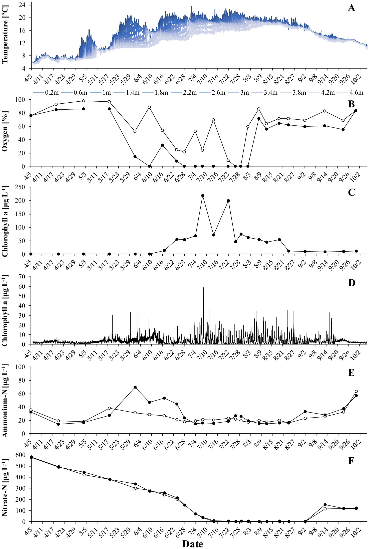
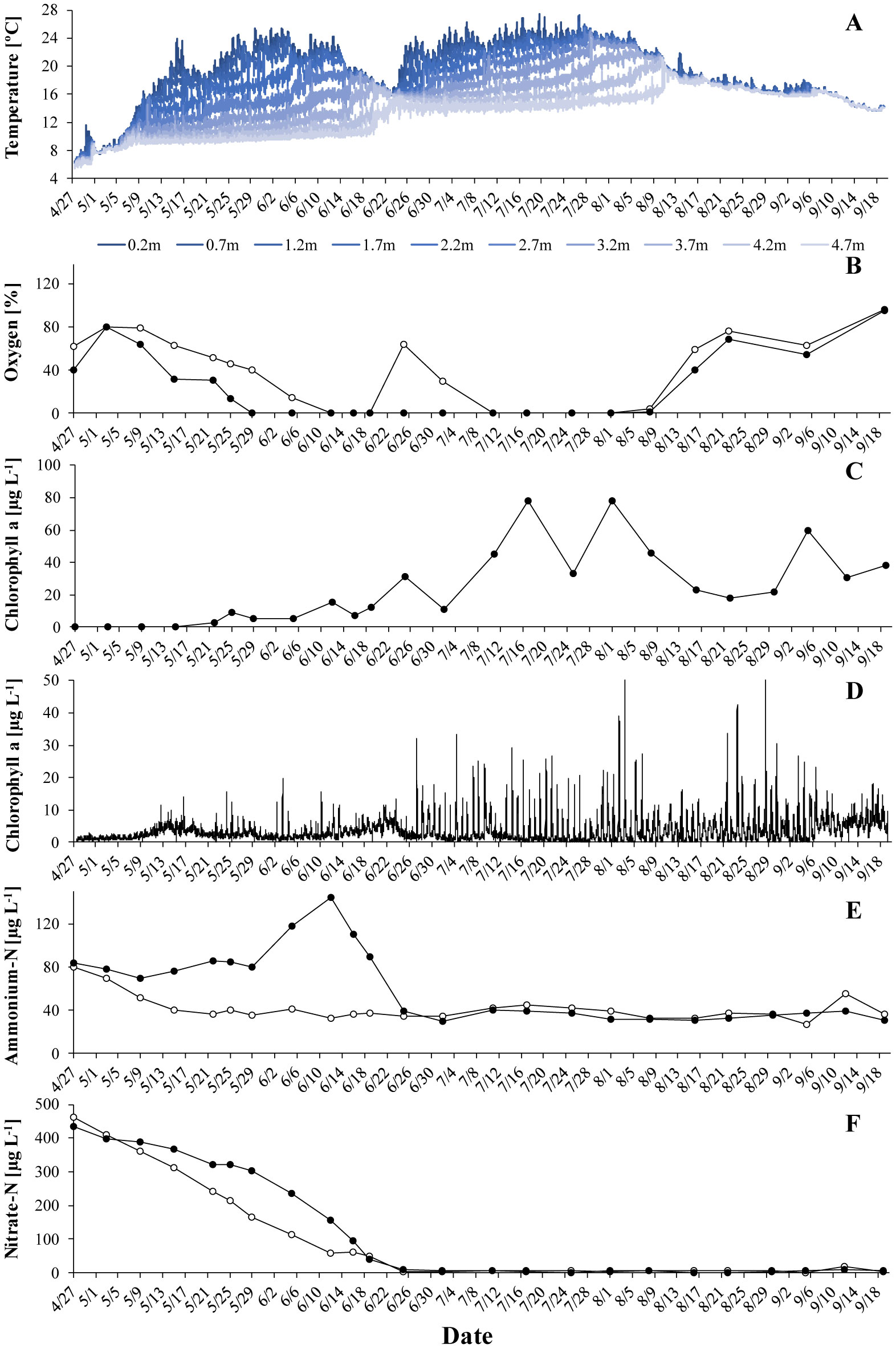
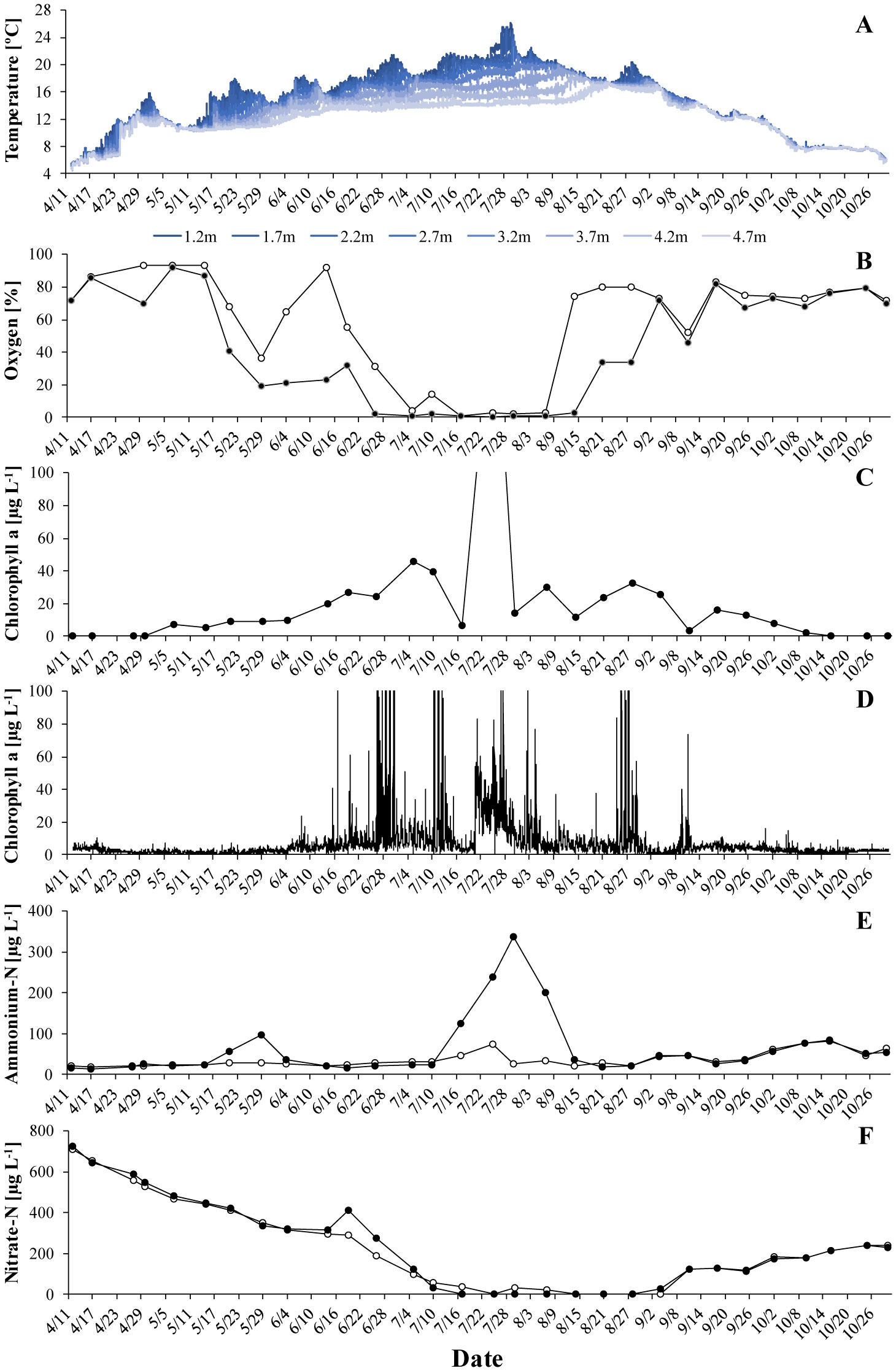
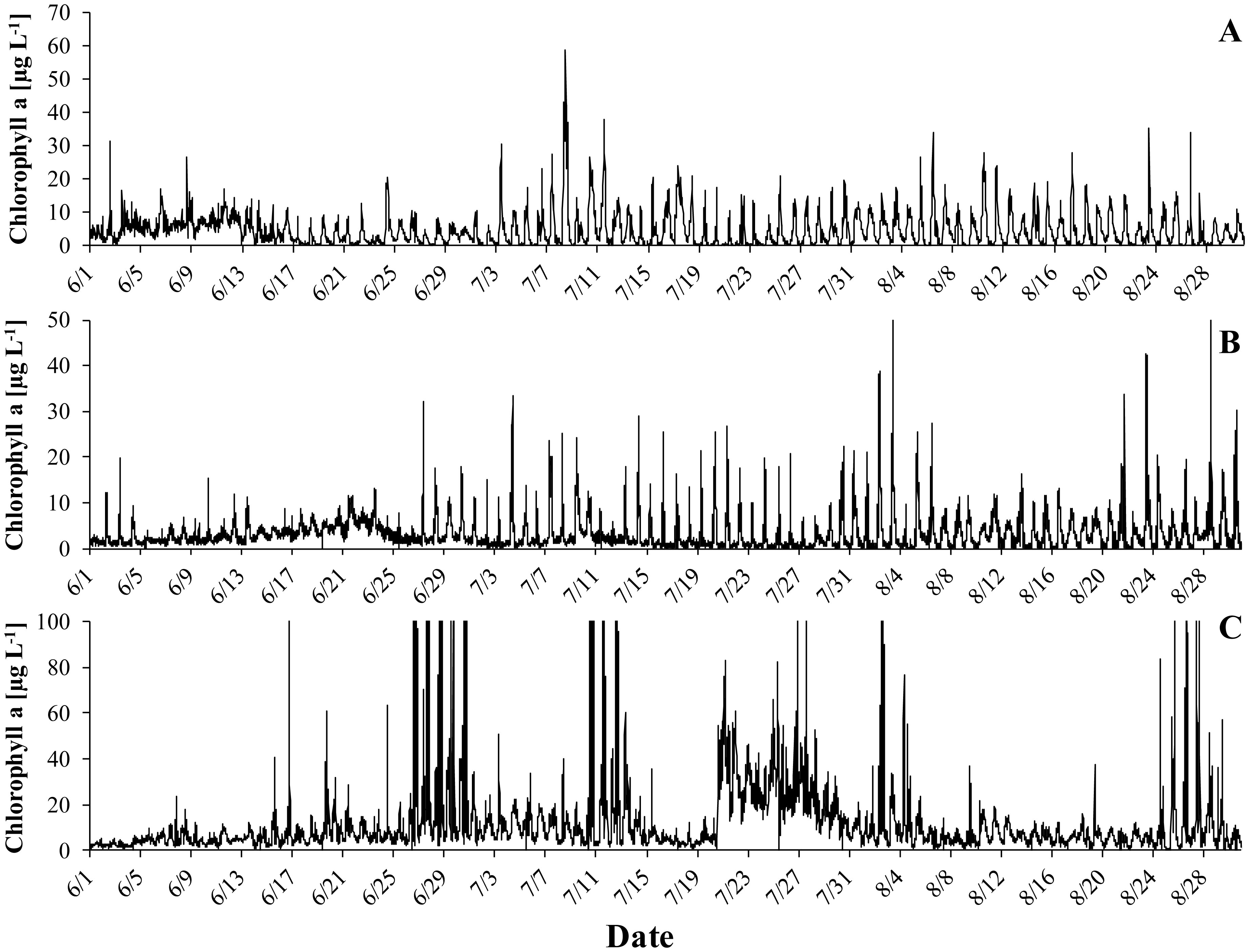
Gonyostomum semen is a bloom-forming freshwater raphidophyte that is currently on the increase, which concerns water managers and ecologists alike. Much indicates that the recent success of G. semen is linked to its diel vertical migration (DVM), which helps to overcome the spatial separation of optimal light conditions for photosynthesis at the surface of a lake and the high concentration of phosphate in the hypolimnion. I here present data from a field study conducted in Lake Lundebyvannet (Norway) in 2017–2019 that are consistent with the idea that the DVM of G. semen also allows for a hypolimnetic uptake of ammonium. As expected, microbial mineralization of organic matter in a low-oxygen environment led to an accumulation of ammonium in the hypolimnion as long as G. semen was absent. In contrast, a decreasing or constantly lower concentration of hypolimnetic ammonium was found in presence of a migrating G. semen population. In summer of 2019, a short break in the DVM of G. semen coincided with a rapid accumulation of hypolimnetic ammonium, which was equally rapidly decimated when G. semen resumed its DVM. Taken together, these data support the idea that G. semen can exploit the hypolimnetic pool of ammonium, which may be one reason for the recent success of the species and its significant impact on the structure of the aquatic food web.
- Gonyostomum semen,
- hypolimnetic ammonium uptake,
- algal blooms, harmful algae,
- nutrient recycling
Citation: Thomas Rohrlack. Hypolimnetic assimilation of ammonium by the nuisance alga Gonyostomum semen[J]. AIMS Microbiology, 2020, 6(2): 92-105. doi: 10.3934/microbiol.2020006

Related Papers:

Abstract

Gonyostomum semen is a bloom-forming freshwater raphidophyte that is currently on the increase, which concerns water managers and ecologists alike. Much indicates that the recent success of G. semen is linked to its diel vertical migration (DVM), which helps to overcome the spatial separation of optimal light conditions for photosynthesis at the surface of a lake and the high concentration of phosphate in the hypolimnion. I here present data from a field study conducted in Lake Lundebyvannet (Norway) in 2017–2019 that are consistent with the idea that the DVM of G. semen also allows for a hypolimnetic uptake of ammonium. As expected, microbial mineralization of organic matter in a low-oxygen environment led to an accumulation of ammonium in the hypolimnion as long as G. semen was absent. In contrast, a decreasing or constantly lower concentration of hypolimnetic ammonium was found in presence of a migrating G. semen population. In summer of 2019, a short break in the DVM of G. semen coincided with a rapid accumulation of hypolimnetic ammonium, which was equally rapidly decimated when G. semen resumed its DVM. Taken together, these data support the idea that G. semen can exploit the hypolimnetic pool of ammonium, which may be one reason for the recent success of the species and its significant impact on the structure of the aquatic food web.

Acknowledgment

The author thanks Johnny Kristiansen and Pia Frostad for their assistance in the field and laboratory. The study was supported by NMBU grant 1750051444.

Conflict of interest

The author declares no conflict of interests.

References

[1]	Pęczuła W, Poniewozik M, Szczurowska A (2013) Gonyostomum semen (Ehr.) Diesing bloom formation in nine lakes of Polesie region (Central-Eastern Poland). Annales De Limnologie-Int J Limnol 49: 301-308. doi: 10.1051/limn/2013059
[2]	Findlay D, Paterson J, Hendzel L, et al. (2005) Factors influencing Gonyostomum semen blooms in a small boreal reservoir lake. Hydrobiologia 533: 243-252. doi: 10.1007/s10750-004-2962-z
[3]	Takemoto Y, Furumoto K, Tada A (2002) Diel vertical migration of Gonyostomum semen (Raphidophyceae) in Kawahara lake. Proc Hydraul Eng 46: 1061-1066. doi: 10.2208/prohe.46.1061
[4]	Cowles R, Brambel C (1936) A study of the environmental conditions in a bog pond with special reference to the diurnal vertical distribution of Gonyostomum semen. Biol Bull 71: 286-298. doi: 10.2307/1537435
[5]	Karosienė J, Kasperovičienė J, Koreivienė J, et al. (2014) Assessment of the vulnerability of Lithuanian lakes to expansion of Gonyostomum semen (Raphidophyceae). Limnologica 45: 7-15. doi: 10.1016/j.limno.2013.10.005
[6]	Hagman CHC, Ballot A, Hjermann DO, et al. (2015) The occurrence and spread of Gonyostomum semen (Ehr.) Diesing (Raphidophyceae) in Norwegian lakes. Hydrobiologia 744: 1-14. doi: 10.1007/s10750-014-2050-y
[7]	Lepistö L, Antikainen S, Kivinen J (1994) The occurrence of Gonyostomum semen (EHR) in Finnish lakes. Hydrobiologia 273: 1-8. doi: 10.1007/BF00126764
[8]	Rengefors K, Weyhenmeyer GA, Bloch I (2012) Temperature as a driver for the expansion of the microalga Gonyostomum semen in Swedish lakes. Harmful Algae 18: 65-73. doi: 10.1016/j.hal.2012.04.005
[9]	Trigal C, Hallstan S, Johansson KSL, et al. (2013) Factors affecting occurrence and bloom formation of the nuisance flagellate Gonyostomum semen in boreal lakes. Harmful Algae 27: 60-67. doi: 10.1016/j.hal.2013.04.008
[10]	Cronberg G, Lindmark G, Björk S (1988) Mass development of the flagellate Gonyostomum semen (Raphidophyta) in Swedish forest lakes-an effect of acidification? Hydrobiologia 161: 217-236. doi: 10.1007/BF00044113
[11]	Münzner K (2019) Gonyostomum semen i svenska sjöar-förekomst och problem Uppsala University, Limnology, 16.
[12]	Rakko A, Laugaste R, Ott I (2008) Algal blooms in Estonian small lakes. Algal Toxins: Nature, Occurrence, Effect and Detection Springer, 211-220. doi: 10.1007/978-1-4020-8480-5_8
[13]	Hongve D, Løvstad Ø, Bjørndalen K (1988) Gonyostomum semen—a new nuisance to bathers in Norwegian lakes: With 4 figures in the text. Int Vereinigung für theoretische und angewandte Limnologie: Verhandlungen 23: 430-434.
[14]	Johansson KS, Trigal C, Vrede T, et al. (2016) Algal blooms increase heterotrophy at the base of boreal lake food webs - evidence from fatty acid biomarkers. Limnol Oceanogr 61: 1563-1573. doi: 10.1002/lno.10296
[15]	Johansson KS, Trigal C, Vrede T, et al. (2013) Community structure in boreal lakes with recurring blooms of the nuisance flagellate Gonyostomum semen. Aquat sci 75: 447-455. doi: 10.1007/s00027-013-0291-x
[16]	Lebret K, Fernández Fernández M, Hagman CH, et al. (2012) Grazing resistance allows bloom formation and may explain invasion success of Gonyostomum semen. Limnol Oceanogr 57: 727-734. doi: 10.4319/lo.2012.57.3.0727
[17]	Trigal C, Goedkoop W, Johnson RK (2011) Changes in phytoplankton, benthic invertebrate and fish assemblages of boreal lakes following invasion by Gonyostomum semen. Freshwater Biol 56: 1937-1948. doi: 10.1111/j.1365-2427.2011.02615.x
[18]	Salonen K, Rosenberg M (2000) Advantages from diel vertical migration can explain the dominance of Gonyostomum semen (Raphidophyceae) in a small, steeply-stratified humic lake. J Plankton Res 22: 1841-1853. doi: 10.1093/plankt/22.10.1841
[19]	Rohrlack T (2019) The diel vertical migration of the nuisance alga Gonyostomum semen is controlled by temperature and by a circadian clock. Limnologica 80: 125746. doi: 10.1016/j.limno.2019.125746
[20]	Eloranta P, Räike A (1995) Light as a factor affecting the vertical distribution of Gonyostomum semen(Ehr.) Diesing(Raphidophyceae) in lakes. Aqua Fennica(name change effective with 1996 issues) 25: 15-22.
[21]	Hessen DO, Hall JP, Thrane JE, et al. (2017) Coupling dissolved organic carbon, CO₂ and productivity in boreal lakes. Freshwater Biol 62: 945-953. doi: 10.1111/fwb.12914
[22]	Thrane J-E, Hessen DO, Andersen T (2014) The absorption of light in lakes: negative impact of dissolved organic carbon on primary productivity. Ecosystems 17: 1040-1052. doi: 10.1007/s10021-014-9776-2
[23]	Watanabe M, Kohata K, Kimura T (1991) Diel vertical migration and nocturnal uptake of nutrients by Chattonella antiqua under stable stratification. Limnol Oceanogr 36: 593-602. doi: 10.4319/lo.1991.36.3.0593
[24]	Dortch Q, Maske M (1982) Dark uptake of nitrate and nitrate reductase activity of a red-tide population off peru. Mar Ecol Prog Ser 9: 299-303. doi: 10.3354/meps009299
[25]	Bhovichitra M, Swift E (1977) Light and dark uptake of nitrate and ammonium by large oceanic dinoflagellates: Pyrocystis noctiluca, Pyrocystis fusiformis, and Dissodinium lunula. Limnol Oceanogr 22: 73-83. doi: 10.4319/lo.1977.22.1.0073
[26]	Fernandez E, Galvan A (2008) Nitrate assimilation in Chlamydomonas. Eukaryotic Cell 7: 555-559. doi: 10.1128/EC.00431-07
[27]	Sinclair GA, Kamykowski D, Milligan E, et al. (2006) Nitrate uptake by Karenia brevis. I. Influences of prior environmental exposure and biochemical state on diel uptake of nitrate. Mar Ecol Prog Ser 328: 117-124. doi: 10.3354/meps328117
[28]	Lieberman OS, Shilo M, van Rijn J (1994) The physiological ecology of a freshwater dinoflagellate bloom population: Vertical migration, nitrogen limitation and nutrient uptake kinetics. J Phycol 30: 964-971. doi: 10.1111/j.0022-3646.1994.00964.x
[29]	Labib W (1995) Diel vertical migration and toxicity of Alexandrium minutum Halim red tide, in Alexandria, Egypt. Mar Life 5: 11-17.
[30]	del Giorgio PA, Peters RH (1994) Patterns in planktonic P: R ratios in lakes: influence of lake trophy and dissolved organic carbon. Limnol Oceanogr 39: 772-787. doi: 10.4319/lo.1994.39.4.0772
[31]	Prairie YT, Bird DF, Cole JJ (2002) The summer metabolic balance in the epilimnion of southeastern Quebec lakes. Limnol Oceanogr 47: 316-321. doi: 10.4319/lo.2002.47.1.0316
[32]	Hanson PC, Bade DL, Carpenter SR, et al. (2003) Lake metabolism: relationships with dissolved organic carbon and phosphorus. Limnol Oceanogr 48: 1112-1119. doi: 10.4319/lo.2003.48.3.1112
[33]	Sobek S, Algesten G, Bergstrøm A-K, et al. (2003) The catchment and climate regulation of pCO₂ in boreal lakes. Global Change Biol 9: 630-641. doi: 10.1046/j.1365-2486.2003.00619.x
[34]	Syrett P, Leftley J (2016) Nitrate and urea assimilation by algae. Perspec Exp Biol 2: 221-234.
[35]	Xiao Y, Rohrlack T, Riise G (2020) Unraveling long-term changes in lake color based on optical properties of lake sediment. Sci Total Environ 699: 134388. doi: 10.1016/j.scitotenv.2019.134388
[36]	Hagman CHC, Rohrlack T, Uhlig S, et al. (2019) Heteroxanthin as a pigment biomarker for Gonyostomum semen (Raphidophyceae). PloS one 14: e0226650. doi: 10.1371/journal.pone.0226650
[37]	Wright SW, Jeffrey SW, Mantoura RFC, et al. (1991) Improved HPLC method for the analysis of chlorophylls and caroteniods from marine phytoplankton. Mar Ecol Prog Ser 77: 183-196. doi: 10.3354/meps077183
[38]	Eppley RW, Rogers JN, McCarthy JJ, et al. (1969) Half-saturation constants for uptake of nitrate and ammonium by marine phytoplankton. J Limnology 14: 912-920.
[39]	Nakamura Y (1985) Ammonium uptake kinetics and interactions between nitrate and ammonium uptake in Chattonella antiqua. J Oceanogr Soci Jpn 41: 33-38. doi: 10.1007/BF02109929
[40]	Fisher T, Morrissey K, Carlson P, et al. (1988) Nitrate and ammonium uptake by plankton in an Amazon River floodplain lake. J Plankton Res 10: 7-29. doi: 10.1093/plankt/10.1.7
[41]	Reay DS, Nedwell DB, Priddle J, et al. (1999) Temperature dependence of inorganic nitrogen uptake: reduced affinity for nitrate at suboptimal temperatures in both algae and bacteria. Appl Environ Microbiol 65: 2577-2584. doi: 10.1128/AEM.65.6.2577-2584.1999
[42]	Nicklisch A, Kohl JG (1983) Growth kinetics of Microcystis aeruginosa (Kütz) Kütz as a basis for modelling its population dynamics. Int Revue der gesamten Hydrobiologie und Hydrographie 68: 317-326. doi: 10.1002/iroh.19830680304
[43]	Johansson KS, Vrede T, Lebret K, et al. (2013) Zooplankton feeding on the nuisance flagellate Gonyostomum semen. PloS one 8.
[44]	Pęczuła W (2007) Mass development of the algal species Gonyostomum semen (Raphidophyceae) in the mesohumic Lake Płotycze (central-eastern Poland). Hydrobiol Stud 36: 163-172.
[45]	Ibelings BW, Maberly SC (1998) Photoinhibition and the availability of inorganic carbon restrict photosynthesis by surface blooms of cyanobacteria. Limnol Oceanogr 43: 408-419. doi: 10.4319/lo.1998.43.3.0408
[46]	Jonsson A, Karlsson J, Jansson M (2003) Sources of carbon dioxide supersaturation in clearwater and humic lakes in northern Sweden. Ecosystems 6: 224-235. doi: 10.1007/s10021-002-0200-y
[47]	Sobek S, Tranvik LJ, Cole JJ (2005) Temperature independence of carbon dioxide supersaturation in global lakes. Global Biogeochem Cycles 19. doi: 10.1029/2004GB002264
[48]	Whitfield CJ, Seabert TA, Aherne J, et al. (2010) Carbon dioxide supersaturation in peatland waters and its contribution to atmospheric efflux from downstream boreal lakes. J Geophys Res 115.
[49]	Hagman CHC, Skjelbred B, Thrane J-E, et al. (2019) Growth responses of the nuisance algae Gonyostomum semen (Raphidophyceae) to DOC and associated alterations of light quality and quantity. Aquat Microb Ecol 82: 241-251. doi: 10.3354/ame01894
[50]	Lebret K, Östman Ö, Langenheder S, et al. (2018) High abundances of the nuisance raphidophyte Gonyostomum semen in brown water lakes are associated with high concentrations of iron. Sci Rep 8: 13463. doi: 10.1038/s41598-018-31892-7