Citation: Zachary Abernathy, Kristen Abernathy, Jessica Stevens. A mathematical model for tumor growth and treatment using virotherapy[J]. AIMS Mathematics, 2020, 5(5): 4136-4150. doi: 10.3934/math.2020265

| [1] | US Department of Health and Human Services, Nci dictionary of cancer terms, Available from: https://www.cancer.gov/publications/dictionaries/cancer-terms?cdrid=457964. |
| [2] | Virotherapy.eu. About virotherapy, Available from: https://www.virotherapy.com/treatment.php. |
| [3] | Virotherapy.eu. Treatment, Available from: https://www.virotherapy.com/treatment.php. |
| [4] | M. D. Liji Thomas, What is virotherapy? 2015. Available from: https://www.news-medical.net/health/What-is-Virotherapy.aspx.%7D%7Bwww.news-medical.net/health/What-is-Virotherapy.aspx. |
| [5] |
S. J. Russell, K. Peng, J. C. Bell, Oncolytic virotherapy, Nat. biotechnol., 30 (2012), 658-670. doi: 10.1038/nbt.2287

|
| [6] | S. X. staff, First study of oncolytic hsv-1 in children and young adults with cancer indicates safety, tolerability, 2017. Available from: https://medicalxpress.com/news/2017-05-oncolytic-hsv-children-young-adults.html. |
| [7] | K. A. Streby, J. I. Geller, M. A. Currier, et al. Intratumoral injection of hsv1716, an oncolytic herpes virus, is safe and shows evidence of immune response and viral replication in young cancer patients, 2017. Available from: http://clincancerres.aacrjournals.org/content/early/2017/05/10/1078-0432.CCR-16-2900. |
| [8] | T. Tadesse, A. Bekuma, A promising modality of oncolytic virotherapy for cancer treatment, J. Vet. Med. Res., 5 (2018), 1163. |
| [9] | A. Reale, A. Vitiello, V. Conciatori, et al. Perspectives on immunotherapy via oncolytic viruses, Infect. agents canc., 14 (2016), 5. |
| [10] | M. Agarwal, A. S. Bhadauria, et al. Mathematical modeling and analysis of tumor therapy with oncolytic virus. Appl. Math., 2 (2011), 131. |
| [11] |
J. Malinzi, P. Sibanda, H. Mambili-Mamboundou, Analysis of virotherapy in solid tumor invasion, Math. Biosci., 263 (2015), 102-110. doi: 10.1016/j.mbs.2015.01.015
|
| [12] |
M. J. Piotrowska, An immune system-tumour interactions model with discrete time delay: Model analysis and validation, Commu. Nonlinear Sci., 34 (2016), 185-198. doi: 10.1016/j.cnsns.2015.10.022
|
| [13] | A. Friedman, X. Lai, Combination therapy for cancer with oncolytic virus and checkpoint inhibitor: A mathematical model, PloS one, 13 (2018), e0192449. |
| [14] | A. L. Jenner, A. C. F. Coster, P. S. Kim, et al. Treating cancerous cells with viruses: insights from a minimal model for oncolytic virotherapy, Lett. Biomath., 5 (2018), S117-S136. |
| [15] |
A. L. Jenner, C. Yun, P. S. Kim, et al. Mathematical modelling of the interaction between cancer cells and an oncolytic virus: Insights into the effects of treatment protocols, B. Math. Biol., 80 (2018), 1615-1629. doi: 10.1007/s11538-018-0424-4
|
| [16] |
D. Wodarz, Computational modeling approaches to the dynamics of oncolytic viruses, Wiley Interdiscip. Rev.: Syst. Biol. Med., 8 (2016), 242-252. doi: 10.1002/wsbm.1332
|
| [17] |
P. S. Kim, J. J. Crivelli, I. Choi, et al. Quantitative impact of immunomodulation versus oncolysis with cytokine-expressing virus therapeutics, Math. Biosci. Eng., 12 (2015), 841-858. doi: 10.3934/mbe.2015.12.841
|
| [18] | M. Nowak, R. M. May, Virus dynamics: Mathematical principles of immunology and virology: Mathematical principles of immunology and virology, Oxford University Press, UK, 2000. |
| [19] | J. Guckenheimer, P. Holmes, Nonlinear oscillations, dynamical systems, and bifurcations of vector fields, Springer Science Business Media, 2013. |
| [20] | Y. A. Yuznetsov, Elements of Applied Bifurcation Theory, Springer, 2004. |
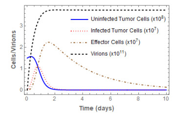
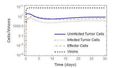
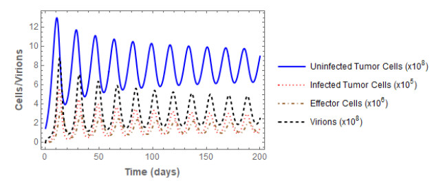
Figures(3) / Tables(2)

Zachary Abernathy, Kristen Abernathy, Jessica Stevens. A mathematical model for tumor growth and treatment using virotherapy[J]. AIMS Mathematics, 2020, 5(5): 4136-4150. doi: 10.3934/math.2020265


 DownLoad: