
Citation: Chunhong Li, Sanxing Liu. Stochastic invariance for hybrid stochastic differential equation with non-Lipschitz coefficients[J]. AIMS Mathematics, 2020, 5(4): 3612-3633. doi: 10.3934/math.2020234
[1] | Rania Abozahra, Amal Gaballah, Sarah M. Abdelhamid . Prevalence of the colistin resistance gene MCR-1 in colistin-resistant Klebsiella pneumoniae in Egypt. AIMS Microbiology, 2023, 9(2): 177-194. doi: 10.3934/microbiol.2023011 |
[2] | Kholoud Baraka, Rania Abozahra, Marwa Mohammed Haggag, Sarah M Abdelhamid . Genotyping and molecular investigation of plasmid-mediated carbapenem resistant clinical Klebsiella pneumoniae isolates in Egypt. AIMS Microbiology, 2023, 9(2): 228-244. doi: 10.3934/microbiol.2023014 |
[3] | Amira H. El-Ashry, Shimaa R. Hendawy, Noha Mostafa Mahmoud . Prevalence of pks genotoxin among hospital-acquired Klebsiella pneumoniae. AIMS Microbiology, 2022, 8(1): 73-82. doi: 10.3934/microbiol.2022007 |
[4] | Sunarno Sunarno, Nelly Puspandari, Fitriana Fitriana, Uly Alfi Nikmah, Hasta Handayani Idrus, Novaria Sari Dewi Panjaitan . Extended spectrum beta lactamase (ESBL)-producing Escherichia coli and Klebsiella pneumoniae in Indonesia and South East Asian countries: GLASS Data 2018. AIMS Microbiology, 2023, 9(2): 218-227. doi: 10.3934/microbiol.2023013 |
[5] | Ogueri Nwaiwu, Chiugo Claret Aduba . An in silico analysis of acquired antimicrobial resistance genes in Aeromonas plasmids. AIMS Microbiology, 2020, 6(1): 75-91. doi: 10.3934/microbiol.2020005 |
[6] | Rochelle Keet, Diane Rip . Listeria monocytogenes isolates from Western Cape, South Africa exhibit resistance to multiple antibiotics and contradicts certain global resistance patterns. AIMS Microbiology, 2021, 7(1): 40-58. doi: 10.3934/microbiol.2021004 |
[7] | Amira ElBaradei, Dalia Ali Maharem, Ola Kader, Mustafa Kareem Ghareeb, Iman S. Naga . Fecal carriage of ESBL-producing Escherichia coli in Egyptian patients admitted to the Medical Research Institute hospital, Alexandria University. AIMS Microbiology, 2020, 6(4): 422-433. doi: 10.3934/microbiol.2020025 |
[8] | Taish Ramkisson, Diane Rip . Carbapenem resistance in Enterobacterales from agricultural, environmental and clinical origins: South Africa in a global context. AIMS Microbiology, 2023, 9(4): 668-691. doi: 10.3934/microbiol.2023034 |
[9] | Alfred Mitema, Naser Aliye Feto . Molecular and Vegetative Compatibility Groups Characterization of Aspergillus flavus Isolates from Kenya. AIMS Microbiology, 2020, 6(3): 231-249. doi: 10.3934/microbiol.2020015 |
[10] | Abdullahi Yusuf Muhammad, Malik Amonov, Chandrika Murugaiah, Atif Amin Baig, Marina Yusoff . Intestinal colonization against Vibrio cholerae: host and microbial resistance mechanisms. AIMS Microbiology, 2023, 9(2): 346-374. doi: 10.3934/microbiol.2023019 |
The study of a hyperplane arrangement typically goes along with the study of its characteristic polynomial as the polynomial carries combinatorial and topological information of the arrangement (e.g., [10,16,17]). Terao's factorization theorem shows that if an arrangement is free, then its characteristic polynomial factors into the product of linear polynomials over the integer ring. Many attempts have been made in order to compute and to make a broader understanding the characteristic polynomials (e.g., [1,2,6,7,9,12,13,15,23,24]). It is well-known that the characteristic polynomial of any hyperplane arrangement gets generalized to the Tutte polynomial [22]. More recently, the generalizations of the polynomials, the arithmetic Tutte polynomial, the characteristic quasi-polynomial and the chromatic quasi-polynomials were introduced (e.g., [12,14,15,21]).
The braid arrangement (or type A Coxeter arrangement) is the hyperplane arrangement in Rn defined by
An−1:={xi−xj=0:1≤i<j≤n}. |
Deformations of the braid arrangement are often studied in the literature, among these deformations are the Linial arrangement, Shi arrangement, Catalan arrangement, semiorder arrangement, generic braid arrangement, and semigeneric braid arrangement, etc, see [3,4,5,8,11,19,20,23] for a discussion of the combinatorics and freeness of these arrangements. The semigeneric braid arrangement is the hyperplane arrangement in Rn defined by
Sn:={xi−xj=ai:1≤i<j≤n}, |
where ai′s are generic. Stanley asked to find the characteristic polynomial of this arrangement. In this paper, we give a formula for the characteristic polynomials of the semigeneric braid arrangement and its subarrangements, which we call the semigeneric graphical arrangements.
The remainder of the paper is organized as follows. In Section 2, we recall definitions and basic facts of arrangements. In Section 3, we prove our main results which provide the characterizations of a central semigeneric graphical arrangement, and induce a formula for the characteristic polynomial of a semigeneric graphical arrangement. In Section 4, we show some applications of our main results.
We first review some basic concepts and preliminary results on arrangements. Our standard reference is [17,18]. Let K be a field, n be a positive integer and V=Kn be the n-dimensional vector space over K. A hyperplane in V is a affine subspace of codimension one of V. An arrangement A is a finite set of hyperplanes in V. An intersection lattice L(A) of A is defined by
L(A):={⋂H∈BH≠∅:B⊆A}, |
with an order by reverse inclusion X≤Y⇔Y⊆X for X,Y∈L(A). The characteristic polynomial χA(t)∈Z[t] of A is defined by
χA(t):=∑X∈L(A)μ(X)tdimX, |
where μ denotes the Möbius function μ:L(A)→Z defined recursively by
μ(V)=1andμ(X)=−∑Y∈L(A)X⊊Yμ(Y). |
Let G be a simple graph with vertex set V(G)=[n]={1,…,n} and edge set E(G). The graphical arrangement AG in Kn is defined by
AG:={xi−xj=0:ij∈E(G)}. |
A simple graph is chordal if it does not contain an induced cycle of length greater than three, or Cn-free for all n>3 in shorthand notation. The freeness of graphical arrangements is completely characterized by chordality. If G=Kn, the complete graph on [n], then AG=An−1.
A natural deformation of the graphical arrangement turns up if we use generic elements ai′s to replace 0′s in the equations of hyperplanes. Stanley explained the meaning of generic elements in [18] as follows.
Let A be an arrangement in an n-dimensional vector space V and L1(x),…,Lm(x) be linear forms, not necessarily distinct, in the variables x=(x1,…,xn) over the field K. Let A be defined by L1(x)=a1,…,Lm(x)=am, where a1,…,am are generic elements of K. This means if Hi=ker(Li(x)−ai), then
Hi1∩⋯∩Hik≠∅⟺Li1,…,Likare linearly independent. |
Definition 2.1. Let G be a simple graph with vertex set V(G)=[n] and edge set E(G). The semigeneric graphical arrangement in Rn is defined by
SG:={xi−xj=ai:ij∈E(G),1≤i<j≤n}, |
where ai′s are generic. SG is simply a subarrangement of the semigeneric braid arrangement Sn. In particular, if G=Kn, then SG=Sn.
According to the definitions of generic elements and SG, the genericity of ai′s can be sure when they take any numbers in R. We do not emphasize that ai′s are generic in later section.
Clearer comprehending can be achieved by a simple example.
Example 2.2. Figure 1 shows a simple graph G, a subgraph of K6, the semigeneric graphical arrangement SG consists of the following hyperplanes:
x1−x2=a1,x1−x5=a1,x2−x3=a2,x2−x4=a2,x2−x5=a2,x2−x6=a2,x3−x4=a3,x3−x5=a3,x4−x6=a4. |
There are a few powerful methods for computing the characteristic polynomials of hyperplane arrangements. In [7], Athanasiadis showed that simply by computing the number of points missing the hyperplanes (over finite fields) and by using the Möbius formula, the characteristic polynomials of many hyperplane arrangements can be computed. Our method is closer in spirit to [18] in which Stanley gives an interpretation of linearly independent subarrangement B of the generic braid arrangement in terms of the graph GB. We will provide a necessary and sufficient condition for a central semigeneric graphical arrangement SG from the point of graph G (i.e., Theorem 3.4).
Lemma 3.1. The semigeneric graphical arrangement SG is central (i.e. ∩H∈SGH≠∅) if the graph G is an acyclic graph.
Proof. SG is central if the intersection of all the hyperplanes contains at least one point (x1,…,xn). We can find such an assignment (x1,…,xn) satisfying xi−xj=ai(ij∈E(G)). That can be done by just picking one from xi′s at a time since the graph G is acyclic and ai's are generic.
Owing to Lemma 3.1, we consider the centrality of SG where G is a cycle.
Lemma 3.2. If the arrangement S:={xij−xij+1=bj:1≤ij≤n,j=1,…,k,ik+1=i1}, then S is central if and only if ∑kj=1bj=0.
Proof. The arrangment S is central means there exists at least one point on all the hyperplanes, that is, at least a solution to the system of the equations of all the hyperplanes in S. That means rank(M(S))=rank((¯M(S)), where M(S) and ¯M(S) are the coefficient matrix and augmented matrix of the system of the equations, respectively.
Perform the following series of elementary row operations on M(S) and ¯M(S), we have
P(k,1(1))…P(k,k−1(1))M(S)=(B0)k×k, |
and
P(k,1(1))…P(k,k−1(1))¯M(S)=(Bβ0∑kj=1bj)k×(k+1), |
where B is a (k−1)×k matrix, βT=(b1,…,bk−1), vector 0=(0,…,0)∈Rk, and P(i,j(m)) denotes the elementary matrix by adding m multiple of j-th row of the identity matrix to i-th row of the identity matrix. Distinctly, ∑kj=1bj=0 if and only if rank(¯M(S))=rank(B)=rank(M(S)), that is, the arrangement S is central.
Applying Lemma 3.2 to a semigeneric graphical arrangement, we get the following theorem.
Theorem 3.3. Let G be a k-cycle with V(G)={i1,…,ik}⊆{1,…,n}, the semigeneric graphical arrangement SG consists of the following hyperplanes:
xij−xij+1={aij,ifij<ij+1aij+1,ifij>ij+1. |
The arrangement SG is central if and only if ∑kj=1(−1)δjaij+δj=0, where δj={0,ifij<ij+11,ifij>ij+1.
In the theorem below, we will characterize the central semigeneric graphical arrangement SG in terms of G.
Theorem 3.4. The semigeneric graphical arrangement SG is central if and only if graph G satisfies one of the following two conditions:
(1) G is an acyclic graph;
(2) the semigeneric graphical arrangements of all cycles in G are central.
Proof. Suppose C1,…,Cp are p connected components of G which are not the isolated vertices. If all the subarrangements corresponding to C1,…,Cp are central, then SG is central. Therefore, it suffices to prove SC is central, where C is a connected component of G containing cycles.
Assume |E(C)|=t and SC:={ker(αi⋅x−ai)|1≤i≤t}. Let T be a spanning tree of C which is a tree that contains every vertex of C, then ¯T=C−E(T) is the cotree of T in C. Assume |V(C)|=s, then |V(T)|=s. Since a connected graph with s vertices is a tree if and only if it has s−1 edges, let the normal vectors of the hyperplanes of ST be αu1,…,αus−1. Firstly, we will prove the vectors αu1,…,αus−1 form a basis of span(α1,…,αt), a space spanned by α1,…,αt. By Lemma 3.1, the vectors αu1,…,αus−1 are linearly independent, i.e., rank(αu1,…,αus−1)=s−1. Moreover, by the definition of spanning tree, we know that T+e will generate a cycle D satisfying e∈E(D) for all e∈E(¯T). Assume |E(D)|=k and αv1,…,αvk−1 are the normal vectors of hyperplanes of SD−e, it follows that
αv1,…,αvk−1∈{αu1,…,αus−1}, |
and the normal vector of hyperplane corresponding to e is αvk∈{α1,…,αt}−{αu1,…,αus−1}. Since D is a cycle, αvk is a linear combination of αv1,…,αvk−1, i.e.,
αvk∈span(αv1,…,αvk−1)⊆span(αu1,…,αus−1). |
Since αvk is the normal vector of hyperplane for any e∈E(¯T), hence α1,…,αt∈span(αu1,…,αus−1), and the vectors αu1,…,αus−1 form a basis of span(α1,…,αt).
Let M(SC) and ¯M(SC) be the coefficient matrix and the augmented matrix of the linear system of the hyperplane equations of SC, respectively, that is,
M(SC)=(α1⋮αt)and¯M(SC)=(α1a1⋮⋮αtat). |
Since αu1,…,αus−1 form a basis of span(α1,…,αt) and the semigeneric graphical arrangements of all cycles in G are central, according to Lemma 3.2, ¯M(SC) can be changed as follows by performing the same series of elementary row operations :
(αu1au1⋮⋮αus−1aus−100⋮⋮00). |
So rank(M(SC))=rank(¯M(SC))=s−1, i.e., SC is central.
We complete the proof.
For the characteristic polynomial of an arrangement A in n-dimensional vector space, we adopt Whitney's theorem [18] which gives a basic formula,
χA(t)=∑B⊆ABiscentral(−1)#Btn−rank(B). |
Combining Whitney's theorem and Theorem 3.4, we will give a formula for the characteristic polynomial of the semigeneric graphical arrangement SG.
Corollary 3.5. Let G be a simple graph with V(G)=[n], then the characteristic polynomial of SG is
χSG(t)=∑D(−1)|E(D)|tp(D), |
where D ranges over all spanning subgraphs of G, and D is an acyclic graph or semigeneric graphical arrangements of all cycles in D are central. |E(D)| denotes the number of the edges, and p(D) denotes the number of the connected components of D.
Proof. Assume D is the spanning subgraph of G corresponding to the subarrangement B of SG. It is clear that #B=|E(D)|. The rank of B is the number of the edges of a spanning forest of D. Since a connected graph with n vertices is a tree if and only if it has n−1 edges, the number of the edges of a spanning forest of a graph D is the number of vertices minus the number of connected components, that is rank(B)=n−p(D).
In this section, we will give some applications of Theorem 3.4 and Corollary 3.5.
Example 4.1. The defining polynomial of S4 (i.e., 4-dimensional semigeneric braid arrangement) is
QS4=(x1−x2−a1)(x1−x3−a1)(x1−x4−a1)(x2−x3−a2)(x2−x4−a2)(x3−x4−a3), |
where a1,a2,a3 are generic elements. Table 1 illustrates all types of characteristic polynomials for S4, which depend on the values of a2,a3,a2+a3,a2−a3. The symbol "T" in Table 1 indicates that the condition is met, and "F" indicates that the condition is not met.
a2=0 | a3=0 | a2+a3=0 | a2−a3=0 | χS4(t) |
F | F | F | F | t4−6t3+15t2−15t |
F | F | T / F | F / T | t4−6t3+15t2−14t |
T / F | F / T | F | F | t4−6t3+13t2−10t |
T | T | T | T | t4−6t3+11t2−6t |
Example 4.2. For the semigeneric graphical arrangement SG of Example 2.2, we take a1=1,a2=3,a3=0,a4=2. Compute the characteristic polynomial χSG(t).
According to Theorem 3.4, we need to figure out the central subarrangements of cycles in G, which depend on the values of the generic elements ai′s. In Figure 2, it is not difficult to see the semigeneric graphical arrangements corresponding to cycles (a)–(c) are central, the others are non-central.
Obviously, a subarrangement of SG is central if and only if the corresponding subgraph D is an acyclic graph or only contains cycles (a), (b) or (c) in Figure 2. The isomorphism types of spanning subgraph D (with the number of distinct labelings written below D) are given by Figure 3.
For all the subgraphs D in Figure 3, we will list the number of connected components p(D), the number of edges |E(D)|, and the number of distinct labelings of D in Table 2.
p(D) | type | |E(D)| | the number of distinct labelings of D |
6 | (a) | 0 | 1 |
5 | (b) | 1 | 9 |
4 | (c) | 2 | 36 |
(d), (e) | 3 | 2 | |
3 | (f) | 3 | 80 |
(g), (h), (i) | 4 | 13 | |
(k) | 5 | 1 | |
2 | (j) | 4 | 99 |
(l), (m), (n) | 5 | 30 | |
(p) | 6 | 4 | |
1 | (o) | 5 | 55 |
(q), (r), (s) | 6 | 24 | |
(t) | 7 | 4 |
Hence, from Corollary 3.5, we get
χSG(t)=t6−9t5+(36−2)t4−(80−13+1)t3+(99−30+4)t2−(55−24+4)t=t6−9t5+34t4−68t3+73t2−35t. |
In this paper, we study the characteristic polynomial of the semigeneric graphical arrangement SG, which is a deformation of the graphical arrangement. The formula of the characteristic polynomial is obtained by characterizing central subarrangements of SG via the corresponding graph G. The semigeneric graphical arrangement SG is a subarrangement of the semigeneric braid arrangement (or type A semigeneric arrangement). It would be interesting to develop a new method for computing the characteristic polynomials of others types (e.g., type B and type D) of semigeneric arrangements in the future.
The work was partially supported by Science and Technology Research Project of Jilin Province (No. JJKH20220719KJ) and NSF of China (No. 11501051).
The authors declare no conflict of interest in this paper.
[1] |
X. R. Mao, Stability of stochastic differential equations with Markovian switching, Stoch. Proc. Appl., 79 (1999), 45-67. doi: 10.1016/S0304-4149(98)00070-2
![]() |
[2] | Y. Xu, Z. M. He, P. G. Wang, Pth monent asymptotic stability for neutral stochastic functional diferential equations with Lévy processes, Appl. Math. Comput., 269 (2015), 594-605. |
[3] |
F. Chen, M. X. Shen, W. Y. Fei, et al. Stability of highly nonlinear hybrid stochastic integrodifferential delay equations, Nonlinear Anal. Hybrid Syst., 31 (2019), 180-199. doi: 10.1016/j.nahs.2018.09.001
![]() |
[4] |
J. W. Luo, K. Liu, Stability of infinite dimensional stochastic evolution equations with memory and Markovian jumps, Stoch. Proc. Appl., 118 (2008), 864-895. doi: 10.1016/j.spa.2007.06.009
![]() |
[5] | A. V. Skorokhod, Asymptotic methods in the theory of stochastic differential equations, Providence: American Mathematical Society, 1989. |
[6] |
H. J. Wu, J. T. Sun, p-Moment stability of stochastic differential equations with impulsive jump and Markovian switching, Automatica, 42 (2006), 1753-1759. doi: 10.1016/j.automatica.2006.05.009
![]() |
[7] | E. W. Zhu, X. Tian, Y. H. Wang, On pth moment exponential stability of stochastic differential equations with Markovian switching and time-varying delay, J. Inequal. Appl., 1 (2015), 1-11. |
[8] | X. R. Mao, C. G. Yuan, Stochastic differential equations with Markovian switching, London: Imperial College Press, 2006. |
[9] |
N. T. Dieu, Some results on almost sure stability of non-Autonomous stochastic differential equations with Markovian switching, Vietnam J. Math., 44 (2016), 1-13. doi: 10.1007/s10013-016-0187-x
![]() |
[10] |
L. G. Xu, Z. L. Dai, H. X. Hu, Almost sure and moment asymptotic boundedness of stochastic delay differential systems, Appl. Math. Comput., 361 (2019), 157-168. doi: 10.1016/j.cam.2019.04.001
![]() |
[11] |
A. E. Jaber, B. Bouchard, C. Illand, Stochastic invariance of closed sets with non-Lipschitz coefficients, Stoch. Proc. Appl., 129 (2019), 1726-1748. doi: 10.1016/j.spa.2018.06.003
![]() |
[12] |
D. Cao, C. Y. Sun, M. Yang, Dynamics for a stochastic reaction-diffusion equation with additive noise, J. Differ. Equations, 259 (2015), 838-872. doi: 10.1016/j.jde.2015.02.020
![]() |
[13] |
D. Li, C. Y. Sun, Q. Q. Chang, Global attractor for degenerate damped hyperbolic equations, J. Math. Anal. Appl., 453 (2017), 1-19. doi: 10.1016/j.jmaa.2017.03.077
![]() |
[14] | A. Friedman, Stochastic differential equations and applications, New York: Academic Press, 1975. |
[15] | J. P. Aubin, G. D. Prato, Stochastic viability and invariance, Ann. Scuola. Norm-Sci., 17 (1990), 595-613. |
[16] |
Tappe, Stefan, Invariance of closed convex cones for stochastic partial differential equations, J. Math. Anal. Appl., 451 (2017), 1077-1122. doi: 10.1016/j.jmaa.2017.02.044
![]() |
[17] | I. Chueshov, M. Scheutzow, Invariance and monotonicity for stochastic delay differential equations, Discrete Cont. Dyn-B., 18 (2013), 1533-1554. |
[18] | B. Øksendal, Stochastic differential equations: An introduction with applications, 6 Eds., Bei Jing: World Publishing Corporation, 2003. |
[19] |
D. H. He, L. G. Xu, Boundedness analysis of stochastic integrodifferential systems with Lévy noise, J. Taibah Univ. Sci., 14 (2020), 87-93. doi: 10.1080/16583655.2019.1708540
![]() |
[20] | S. E. A. Mohammed, Stochastic functional differential equations, Boston: Pitman Advanced Publishing Program, 1984. |
[21] |
R. Buckdahn, M. Quincampoix, C. Rainer, Another proof for the equivalence between invariance of closed sets with respect to stochastic and deterministic systems, B. Sci. Math., 134 (2010), 207-214. doi: 10.1016/j.bulsci.2007.11.003
![]() |
[22] |
B. P. Cheridito, H. M. Soner, N. Touzi, Small time path behavior of double stochastic integrals and applications to stochastic control, Ann. Appl. Probab., 15 (2005), 2472-2495. doi: 10.1214/105051605000000557
![]() |
[23] | R. T. Rockafellar, J. B. Wets, Variational analysis, New York: Springer, 1998. |
[24] | G. T. Kurtz, Lectures on stochastic analysis, 2 Eds., Madison: University of Wisconsin-Madison, 2007. |
[25] | S. N. Ethier, T. G. Kurtz, Markov processes: Characterization and convergence, New Jersey: John Wiley and Sons, 1986. |
[26] | C. H. Li, J. W. Luo, Stochastic invariance for neutral functional differential equation with nonLipschitz coefficients, Discrete. Cont. Dyn-B., 24 (2019), 3299-3318. |
[27] | X. R. Mao, Stochastic defferential equations and application, 2 Eds., Chichester: Woodhead Publishing, 2007. |
[28] |
F. K. Wu, S. G. Hu, C. M. Huang, Robustness of general decay stability of nonlinear neutral stochastic functional differential equations with infinite delay, Syst. Control. Lett., 59 (2010), 195-202. doi: 10.1016/j.sysconle.2010.01.004
![]() |
[29] | C. G. Yuan, J. Lygeros, Stochastic markovian switching hybrid processes, Cambridge: University of Cambridge, 2004. |
[30] | L. G. Xu, S. S. Ge, H. X. Hu, Boundedness and stability analysis for impulsive stochastic differential equations driven by G-Brownian motion, Int. J. Control, 92 (2017), 1-16. |
[31] | B. Yang, Z. Zeng, L. Wang, Most probable phase portraits of stochastic differential equations and its numerical simulation, arXiv.org, 2017. Available from: https://arxiv.org/abs/1703.06789. |
[32] | J. R. Magnus, H. Neudecker, Matrix differential calculus with applications in statistics and econometrics, 3 Eds., New Jersey: Wiley, 2007. |
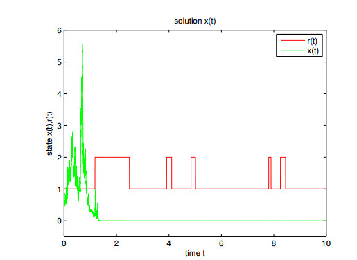
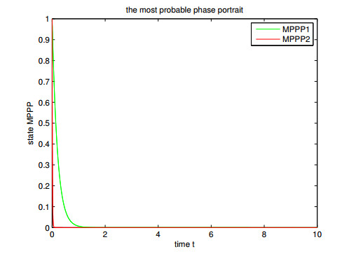
1. | Ruimei Gao, Yuyu Wang, The characteristic polynomials of semigeneric threshold arrangements, 2023, 8, 2473-6988, 28569, 10.3934/math.20231462 |
a2=0 | a3=0 | a2+a3=0 | a2−a3=0 | χS4(t) |
F | F | F | F | t4−6t3+15t2−15t |
F | F | T / F | F / T | t4−6t3+15t2−14t |
T / F | F / T | F | F | t4−6t3+13t2−10t |
T | T | T | T | t4−6t3+11t2−6t |
p(D) | type | |E(D)| | the number of distinct labelings of D |
6 | (a) | 0 | 1 |
5 | (b) | 1 | 9 |
4 | (c) | 2 | 36 |
(d), (e) | 3 | 2 | |
3 | (f) | 3 | 80 |
(g), (h), (i) | 4 | 13 | |
(k) | 5 | 1 | |
2 | (j) | 4 | 99 |
(l), (m), (n) | 5 | 30 | |
(p) | 6 | 4 | |
1 | (o) | 5 | 55 |
(q), (r), (s) | 6 | 24 | |
(t) | 7 | 4 |