


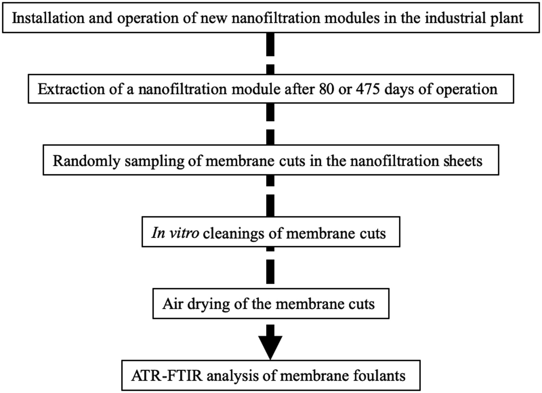
Figure 1.
Flow chart of membrane samples preparation process.
Citation: Carlos García-Padilla, Amelia Aránega, Diego Franco. The role of long non-coding RNAs in cardiac development and disease[J]. AIMS Genetics, 2018, 5(2): 124-140. doi: 10.3934/genet.2018.2.124
| [1] | Mazhyn Skakov, Arman Miniyazov, Victor Baklanov, Alexander Gradoboev, Timur Tulenbergenov, Igor Sokolov, Yernat Kozhakhmetov, Gainiya Zhanbolatova, Ivan Kukushkin . Influence of helium plasma on the structural state of the surface carbide layer of tungsten. AIMS Materials Science, 2023, 10(4): 725-740. doi: 10.3934/matersci.2023040 |
| [2] | Okechukwu Okafor, Abimbola Popoola, Olawale Popoola, Samson Adeosun . Surface modification of carbon nanotubes and their nanocomposites for fuel cell applications: A review. AIMS Materials Science, 2024, 11(2): 369-414. doi: 10.3934/matersci.2024020 |
| [3] | Christian M. Julien, Alain Mauger . Functional behavior of AlF3 coatings for high-performance cathode materials for lithium-ion batteries. AIMS Materials Science, 2019, 6(3): 406-440. doi: 10.3934/matersci.2019.3.406 |
| [4] | Christoph Nick, Helmut F. Schlaak, Christiane Thielemann . Simulation and Measurement of Neuroelectrodes Characteristics with Integrated High Aspect Ratio Nano Structures. AIMS Materials Science, 2015, 2(3): 189-202. doi: 10.3934/matersci.2015.3.189 |
| [5] | Christian M. Julien, Alain Mauger . In situ Raman analyses of electrode materials for Li-ion batteries. AIMS Materials Science, 2018, 5(4): 650-698. doi: 10.3934/matersci.2018.4.650 |
| [6] | Ha Thanh Tung, Ho Kim Dan, Dang Huu Phuc . Effect of the calcination temperature of the FTO/PbS cathode on the performance of a quantum dot-sensitized solar cell. AIMS Materials Science, 2023, 10(3): 426-436. doi: 10.3934/matersci.2023023 |
| [7] | Eugen A. Preoteasa, Elena S. Preoteasa, Ioana Suciu, Ruxandra N. Bartok . Atomic and nuclear surface analysis methods for dental materials: A review. AIMS Materials Science, 2018, 5(4): 781-844. doi: 10.3934/matersci.2018.4.781 |
| [8] | Christian M Julien, Alain Mauger, Ashraf E Abdel-Ghany, Ahmed M Hashem, Karim Zaghib . Smart materials for energy storage in Li-ion batteries. AIMS Materials Science, 2016, 3(1): 137-148. doi: 10.3934/matersci.2016.1.137 |
| [9] | R.A. Silva, C.O. Soares, R. Afonso, M.D. Carvalho, A.C. Tavares, M.E. Melo Jorge, A. Gomes, M.I. da Silva Pereira, C.M. Rangel . Synthesis and electrocatalytic properties of La0.8Sr0.2FeO3−δ perovskite oxide for oxygen reactions. AIMS Materials Science, 2017, 4(4): 991-1009. doi: 10.3934/matersci.2017.4.991 |
| [10] | Shangcong Cheng . On the mechanism of helium permeation through silica glass. AIMS Materials Science, 2024, 11(3): 438-448. doi: 10.3934/matersci.2024022 |
Membrane fouling during filtration is the main limitation of this type of process [1],[2]. Preventive and curative treatments help to limit fouling and to maintain efficient filtration flows [3]–[5]. While inorganic fouling is generally controlled, organic fouling and in particular fouling of biological origin is not. Biofilm development on filtration membrane surfaces, also known as biofouling, is the major fouling component of water filtration systems [5]–[7]. Biofouling is a sequential phenomenon harbouring initial stages of microbial attachment to the membrane and later stages of cell multiplication and extracellular polymeric substances (EPS) production leading to biofilm development [8],[9]. The increase in size of the structure via cell multiplication and the synthesis of matrix corresponds to the stage of maturation of the biofilm. During the maturation process of biofilms formed on nanofiltration (NF) membranes, there is a diversification of the polysaccharide residues of the matrix, development of the polysaccharide network and reinforcement of the cohesion of the matrix by increase of the viscosity and the elasticity [9]. At this stage, shear forces can only tear off a fragment of biofilm when the structure becomes too prominent, limiting the growth of the biofilm in thickness and facilitating the colonization of other sites [10]. Another factor facilitating the geographic expansion of the biofilm is the active detachment of microorganisms that return to the liquid phase [11],[12]. This active detachment involves the production of microbial enzymes to degrade the matrix locally and release sessile bacteria [13].
The biofilm matrix forms a gel structure composed of EPS, mainly polysaccharides, proteins, and nucleic acids and accounts for up to 90% of the dry mass of the biofilm [14]–[17]. In a mature biofilm formed on the surface of nanofiltration membranes in a drinking water production plant, galactoside residues and β-glycan bonds are dominant in the polysaccharide part of the foulants [7]. Peanut agglutinin and wheat germ agglutinin, recognizing the motifs Galβ1-3GalNAcα1-Ser/Thr, and GlcNAcβ1-4GlcNAcβ1-4GlcNAc, respectively, bind strongly to the polysaccharides of the NF biofilm matrix. Other residues are present, and there is some variability in the proportions of the different polysaccharides in the biofilm matrix, depending on the season and the stage of maturity [7],[9]. The matrix polysaccharides are located mainly between cells and organized into entangled fibres of different lengths and cloudy zones. EPS serve as an anchoring cement and protective enclosure for attached microorganisms, rendering mechanical treatments, biocidal treatments and physicochemical treatments less effective [18]. Among the physicochemical treatments against membrane fouling, the acid treatments have a certain efficiency for the release of a part of the fixed inorganic foulants [19]. Alkaline and chelator treatments are more effective than acid treatments in restoring an increased filtration flow [4], [20]–[22]. Alkaline treatments can partially eliminate the biological fouling, fouling associated with natural organic materials and mineral substances. Chelating treatments induce, by the capture of metal ions, the blocking of inorganic, organic and even biological materials. Treatment with anionic surfactants at basic pH shows some cleaning efficiency [23], whereas treatment with cationic surfactants is inconclusive [24]. The anionic surfactant SDS has higher efficiency to remove lipids than polysaccharides and DNA from fouled nanofiltration membranes [25]. Nonionic surfactants reduce the amounts of biofilm and live microorganisms but with limited efficiency [26]. In general, chemical treatments have an interesting efficiency, although partial, but can also induce membrane alterations [27],[28].
Enzyme-containing cleaning solutions can be effective for the treatment of biofilms [29]–[32]. The advantages of the enzymatic treatments are their specificity for a target, the optimal temperatures of use generally not exceeding 50 °C, the pH of optimal use of the order of the physiological pH, a short duration of action if the enzyme concentration is optimal, the biodegradability of enzymes and their limited life in an industrial or natural environment [33]. Thus, enzymatic treatments do not degrade the filtration membranes, and limit additional costs for the treatment of waste. However, since biofilms are complex and heterogeneous, the use of a cleaning solution containing several enzymes seems necessary [7],[34],[35]. In addition, an effective cleaning protocol is usually an association of different products used simultaneously or sequentially [36],[37]. The temperature, the pH, the ionic strength, the concentration of each of the products, their time and their order of application play a key role in the optimization of cleaning processes [22]. Conventional industrial protocols for cleaning nanofiltration membranes use acidic, basic, and detergent solutions [36],[38]. However, these protocols are partially effective, particularly for the removal of biofilm matrix components [35],[39].
In order to identify possibilities for improving the efficiency of commercial cleaning solutions used in nanofiltration membrane practice, we compared the in vitro efficiency of different types of treatments on samples from membranes operating in a drinking water production plant. We used commercial cleaning solutions to which we added or not the two polysaccharidases lactase and pectinase. Both enzymes cleave β-glycan bonds that are widely present in NF biofilms. Lactase cleaves β-D-galactopyranosyl (1→4) β-D-glucopyranose into glucose and galactose. Pectinase contains a polygalacturonase activity and a lower proportion of cellulase activity hydrolyzing respectively the bonds between 2 galactoses in galacturonic acid and glucose polymers. The treatments were tested at two stages of formation of the biofouling deposit corresponding to different levels of maturity of the biofilm.
The flow chart of membrane samples preparation process is shown in Figure 1.
The filtration modules containing new NF200 B-400 membranes (DOW, La Plaine Saint Denis, France) were installed in stage 1 of the integrated pilot at the Méry-sur-Oise industrial plant and extracted after 80 and 475 operating days as previously described [9].
The in vitro cleanings were performed on randomly chosen membrane samples cut of 1 cm2 from an extracted module. Each cleaning protocol was repeated three times on three different membrane coupons. Three static bath cleaning protocols were applied (Table 1). Cleaning protocols were identical for all the steps except a step of application of a different commercial active ingredient. Three types of active ingredients were used. P3-Ultrasil® 110 (Ecolab) is an alkaline detergent treatment (ADT). P3-Ultrasil® 67 (Ecolab) is a neutral liquid detergent containing a combination of stabilized enzymes and surfactants. P3-Ultrasil® 69 (Ecolab) is a mild alkaline liquid detergent containing a combination of organic and inorganic sequestering agents and buffers. The combination of P3-Ultrasil® 67 and P3-Ultrasil® 69 is an alkaline enzymatic detergent treatment (AEDT). Aspergillus oryzae lactase (Sigma-Aldrich, Saint Quentin Fallavier, France), and Aspergillus niger pectinase (Sigma-Aldrich, Saint Quentin Fallavier, France) are two polysaccharidases. Lactase and pectinase associated together to the AEDT treatment was called the multi-enzymatic treatment (MET). The percentages of active products indicated in Table 1 are in volume / volume. Ultrapure water was a bi-distilled water of 18 MΩ quality.
| Alkaline detergent treatment (ADT) | Alkaline enzymatic detergent treatment (AEDT) | Multi-enzymatic treatment (MET) |
| Rinsing with ultrapure water | Rinsing with ultrapure water | Rinsing with ultrapure water |
| P3-Ultrasil® 110 (0.5%) | P3-Ultrasil® 67 (0.5%), P3-Ultrasil® 69 (1%) | Lactase (1%), pectinase (1%) |
| Incubation 4h at 35 °C | Incubation 6h at 39 °C | Incubation 6h at 35 °C |
| Rinsing with ultrapure water at 30 °C | ||
| P3-Ultrasil® 67 (0.5%), P3-Ultrasil® 69 (1%) | ||
| Incubation 6h at 39 °C | ||
| Rinsing with ultrapure water at 30 °C | Rinsing with ultrapure water at 30 °C | Rinsing with ultrapure water at 30 °C |
| Citric acid (0.6%) | Citric acid (0.6%) | Citric acid (0.6%) |
| Incubation 4h at 30 °C | Incubation 4h at 30 °C | Incubation 4h at 30 °C |
| Rinsing with ultrapure water at 30 °C | Rinsing with ultrapure water at 30 °C | Rinsing with ultrapure water at 30 °C |
 DownLoad:
CSV
DownLoad:
CSV
Sample cuts of fouled membranes were air dried for 24h at 40 °C before analysis by ATR-FTIR as previously described [40]. A Tensor 27 IR spectrophotometer with a diamond/ZeSe flat plate crystal (Bruker Optics, Marne la Vallée, France) was used to record IR spectra with air as the background and a resolution of 2 cm−1. Each spectrum presented is the mean of 15 spectra corresponding to different areas of the membrane surface. All the samples were pressed with the same force to obtain equivalent close contact between sample surface and ATR crystal. The membrane IR signal near 700 cm−1 was used to calculate ratio corresponding to the relative IR signals of proteins (band at 1650 cm−1/membrane signal) and polysaccharides (band at 1040 cm−1/membrane signal). Means ± standard deviations of the relative IR signals of proteins and polysaccharides are presented.
The equal-variance Student's t test, following the Fisher's test was used to determine the statistical significance of differences. P values below 0.05, 0.01, or 0.001 were considered significant, highly significant, or very highly significant, respectively.
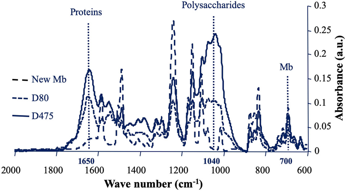
Biofoulants present on the surface of nanofiltration membranes after different filtration times were analysed by ATR-FTIR. IR spectra of fouled membranes are presented in Figure 2 and corresponding relative IR signals of proteins and polysaccharides are presented in Table 2. As observed previously, a certain heterogeneity has been measured between different zones of the membrane, materialized by standard deviations of the relative values of proteins and polysaccharides of the fouling material, which are sometimes high [7],[9]. This emphasizes the importance of collecting fouled membrane samples in different areas and multiplying the IR spectral acquisitions at different points on the surface of each sample. After 80 days of operation (D80), the membrane IR signals were attenuated but the majority of them remained clearly visible. A large quantity of biological macromolecules was accumulated on the surface of the nanofiltration membrane (Figure 2, Table 2). Proteins, materialized by the amide I signal at 1650 cm−1, and polysaccharides materialized by a broad complex region of signals between 1200 and 900 cm−1, were found to be the main foulants as previously described [9],[41]. At D80, the region corresponding to the polysaccharides was composed of 4 peaks around 1080, 1040, 1000 and 970 cm−1. This reveals the diversity of polysaccharide signals at this stage of biofilm development. After 475 days of filtration (D475), the polysaccharide signals became dominant, which shows that at this stage, the biofilm matrix has developed very strongly. The peak at 1040 cm−1 became the major signal among the various polysaccharide signals, as for membranes in operation for several years [35]. Unlike most peaks of the membrane which are largely masked by signals of fouling material at D475, the signal close to 700 cm−1 remains clearly visible, which makes it possible to calculate ratios corresponding to relative IR signals of proteins (1650 cm−1/700 cm−1) and polysaccharides (1040 cm−1/700 cm−1). The means ± standard deviations of the relative IR signals corresponding to the different spectra of membrane samples are presented in Table 2. At D475, compared to D80, the relative values of the IR signals of the proteins did not change significantly, while the relative values of the polysaccharide signals increased significantly. This has already been associated with stagnation of sessile bacterial density and a joint increase of matrix polysaccharides during biofilm growth [9].
| Days of operation (Biofilm age) | Cleaning protocol | Relative IR biofilm signals | |
| Proteins | Polysaccharides | ||
| D80 | - | 2.5 ± 0.1 | 2.2 ± 0.3 |
| D80 | ADT | 1.3 ± 0.3*** | 1.0 ± 0.4*** |
| D80 | AEDT | 1.0 ± 0.3***# | 0.8 ± 0.6*** |
| D80 | MET | 0.9 ± 0.2***## | 0.6 ± 0 .4***# |
| D475 | - | 2.6 ± 1.3 | 3.9 ± 2.3‡‡ |
| D475 | ADT | 1.6 ± 0.6*** | 2.7 ± 1.2** |
| D475 | AEDT | 1.5 ± 0.4*** | 2.7 ± 0.9** |
| D475 | MET | 1.3 ± 0.5***†† | 2.3 ± 1.2**† |
ADT: Alkaline detergent treatment; AEDT: Alkaline enzymatic detergent treatment; MET: Multi-enzymatic treatment; Means and standard deviation of relative IR biofilm signals are presented; ***, **, *: Value differs significantly (
DownLoad:
CSV
Many commercially available cleaning agents can be used for nanofiltration membrane remediation [42]. The inorganic foulants of the deposit accumulated on the filtration membrane is largely eliminated by the current chemical cleanings, which is not the case of the fouling organic material and in particular deposit polysaccharides of the biofilm matrix [35]. It is therefore necessary to carry out efficacy studies of new anti-biofilm cleaning solutions to improve the efficiency of industrial cleaning. Before performing these tests on a large scale, a preliminary in vitro testing step on samples from membranes operating in a water production plant is a good alternative [40]. The effectiveness of three different cleaning protocols according to the use or not of alkaline detergents, surfactants, organic and inorganic sequestering agents, enzymes and in particular polysaccharidases has been evaluated in vitro with the membrane samples described above. The treatments consisted in commercial cleaning solutions, and polysaccharidases.
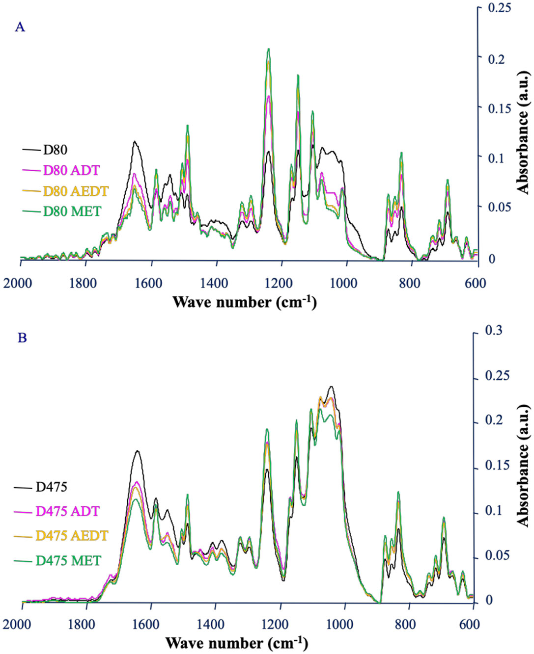
After 80 days of operation, all cleaning protocols had an effect on the biofilm (Figure 3A). Whatever the type of treatment applied, the comparison of the IR spectra before and after cleaning revealed a decrease of the amide I signal and of the band corresponding to the polysaccharides. All the decreases of the foulant signals were significant (Table 2). When comparing the treatments with each other, the alkaline enzymatic detergent treatment (AEDT) was significantly more effective than the alkaline detergent treatment (ADT) in removing proteins but no significant difference in efficacy between the two treatments was observed towards the polysaccharides. The addition of polysaccharidases to AEDT (MET) provided no significant gain in efficiency at this stage of biofilm development. After 475 days of operation, significant decreases in signals of proteins and polysaccharides were also observed on the spectra corresponding to the three treatments compared to no treatment (Figure 3B, Table 2). At this stage, treatments ADT and AEDT had the same efficiency, but the addition of polysaccharidases to treatment AEDT corresponding to treatment MET significantly increased removal of polysaccharides and proteins from the membrane surface. This suggests a reduction of polysaccharides in biofilm biomass after the action of polysaccharidases. A cocktail of polysaccharide-hydrolysing enzymes has been previously shown to remove bacterial biofilm from different solid substrata in laboratory conditions [34]. Alkaline treatments destabilize the microbial membrane, denature proteins and induce the unfolding of extracellular polymeric substances [43]. On the mature biofilm formed after 475 days, the polysaccharidases have a synergistic action with the alkaline enzymatic detergent treatment. Chelating agents, surfactants and enzymes have been previously shown to act synergistically [31]. This synergistic effect could be related to a better diffusion of enzymes within the biofilm during the action of polysaccharidases since the attack of a gel structure like a biofilm by an enzyme is limited by diffusion phenomena [44]. This particular effect associated to polysaccharidases is consistent with the prevalence of polysaccharides in the matrix of NF biofilms formed after 475 days (Figure 3).
There is a need to enhance the efficiency of cleaning procedures to remove biofilms on the surface of nanofiltration membranes used for drinking water production. Despite their efficiency to maintain nanofiltration performance over time through flux recovery, commercial cleaning solutions are only partially efficient against the biofouling deposit. The results presented here showed that polysaccharide-hydrolysing enzymes can increase the in vitro efficiency of a commercially available alkaline enzymatic detergent cleaning solution. Further experiments are needed to characterize the mechanism of this polysaccharidase effect and to confirm this increase of cleaning efficiency in an industrial context.
| [1] |
Carninci P, Kasukawa T, Katayama S, et al. (2005) The transcriptional landscape of the mammalian genome. Science 309: 1559–1563. doi: 10.1126/science.1112014

|
| [2] | Harrow J, Frankish A, Gonzalez JM, et al. (2012). GENCODE: the reference human genome annotation for The ENCODE Project. Genome Res 22: 1760–1774. |
| [3] | Esteller M (2011) Non-coding RNAs in human disease. Nature Rev Gene 12: 861–874. |
| [4] |
Beermann J, Piccoli MT, Viereck J, et al. (2016) Non-coding RNAs in development and disease: background, mechanisms, and therapeutic approaches. Physiol Rev 96: 1297–1325. doi: 10.1152/physrev.00041.2015
|
| [5] |
Barwari T, Joshi A, Mayr M (2016) MicroRNAs in Cardiovascular Disease. J Am College Cardiol 68: 2577–2584. doi: 10.1016/j.jacc.2016.09.945
|
| [6] |
Liu N, Olson EN (2010) MicroRNA regulatory networks in cardiovascular development. Dev Cell 18: 510–525. doi: 10.1016/j.devcel.2010.03.010
|
| [7] |
Derrien T, Johnson R, Bussotti G, et al. (2012) The GENCODE v7 catalog of human long noncoding RNAs: analysis of their gene structure, evolution, and expression. Genome Res 22: 1775–1789. doi: 10.1101/gr.132159.111
|
| [8] | Fang S, Zhang L, Guo J, et al. (2017) NONCODEv5: a comprehensive annotation database for long non coding RNAs. Nucleic Acids Res 46: D308–D314. |
| [9] |
Schmitz SU, Grote P, Herrmann BG (2016) Mechanisms of long noncoding RNA function in development and disease. Cell Mol Life Sci 73: 2491–2509. doi: 10.1007/s00018-016-2174-5
|
| [10] | Rosa A, Ballarino M (2015) Long noncoding RNA regulation of pluripotency. Stem Cells Int 2016: 1–9. |
| [11] |
Wapinski O, Chang HY (2011) Long noncoding RNAs and human disease. Trends in Cell Biol 21: 354–361. doi: 10.1016/j.tcb.2011.04.001
|
| [12] |
Dieci G, Fiorino G, Castelnuovo M, et al. (2007) The expanding RNA polymerase III transcriptome. Trends in Genet 23: 614–622. doi: 10.1016/j.tig.2007.09.001
|
| [13] |
Rackham O, Shearwood AMJ, Mercer TR, et al. (2011) Long noncoding RNAs are generated from the mitochondrial genome and regulated by nuclear-encoded proteins. RNA 17: 2085–2093. doi: 10.1261/rna.029405.111
|
| [14] |
Pauli A, Norris ML, Valen E, et al. (2014) Toddler: an embryonic signal that promotes cell movement via Apelin receptors. Science 343: 1248636. doi: 10.1126/science.1248636
|
| [15] |
Pauli A, Valen E, Schier AF (2015) Identifying (non‐) coding RNAs and small peptides: Challenges and opportunities. BioEssays 37: 103–112. doi: 10.1002/bies.201400103
|
| [16] |
Nelson BR, Makarewich CA, Anderson DM, et al. (2016) A peptide encoded by a transcript annotated as long noncoding RNA enhances SERCA activity in muscle. Science 351: 271–275. doi: 10.1126/science.aad4076
|
| [17] |
Engreitz JM, Ollikainen N, Guttman M (2016) Long non-coding RNAs: spatial amplifiers that control nuclear structure and gene expression. Nat Rev Mol Cell Biol 17: 756–770. doi: 10.1038/nrm.2016.126
|
| [18] |
Gloss BS, Dinger ME (2016) The specificity of long noncoding RNA expression. Biochim Biophysi Acta 1859: 16–22. doi: 10.1016/j.bbagrm.2015.08.005
|
| [19] |
Bär C, Chatterjee S, Thum T (2016) Long Noncoding RNAs in Cardiovascular Pathology, Diagnosis, and Therapy. Circulation 134: 1484–1499. doi: 10.1161/CIRCULATIONAHA.116.023686
|
| [20] |
Chen LL (2016) Linking Long Noncoding RNA Localization and Function. Trends in Biochem Sci 41: 761–772. doi: 10.1016/j.tibs.2016.07.003
|
| [21] |
Klattenhoff CA, Scheuermann JC, Surface LE, et al. (2013) Braveheart, a long noncoding RNA required for cardiovascular lineage commitment. Cell 152: 570–583. doi: 10.1016/j.cell.2013.01.003
|
| [22] |
Ulitsky I, Bartel DP (2013) lincRNAs: genomics, evolution, and mechanisms. Cell 154: 26–46. doi: 10.1016/j.cell.2013.06.020
|
| [23] |
Ounzain S, Pedrazzini T (2015) The promise of enhancer-associated long noncoding RNAs in cardiac regeneration. Trends Cardiovasc Med 25: 592–602. doi: 10.1016/j.tcm.2015.01.014
|
| [24] |
Ounzain S, Burdet F, Ibberson M, et al. (2015) Discovery and functional characterization of cardiovascular long noncoding RNAs. J Mol Cell Cardiol 89: 17–26. doi: 10.1016/j.yjmcc.2015.09.013
|
| [25] |
Memczak S, Jens M, Elefsinioti A, et al. (2013) Circular RNAs are a large class of animal RNAs with regulatory potency. Nature 495: 333–338. doi: 10.1038/nature11928
|
| [26] |
Wang K, Long B, Liu F, et al. (2016) A circular RNA protects the heart from pathological hypertrophy and heart failure by targeting miR-223. Euro Heart J 37: 2602–2611. doi: 10.1093/eurheartj/ehv713
|
| [27] |
Liu L, An X, Li Z, et al. (2016) The H19 long noncoding RNA is a novel negative regulator of cardiomyocyte hypertrophy. Cardiovasc Res 111: 56–65. doi: 10.1093/cvr/cvw078
|
| [28] |
Hasegawa Y, Brockdorff N, Kawano S, et al. (2010) The matrix protein hnRNP U is required for chromosomal localization of Xist RNA. Dev Cell 19: 469–476. doi: 10.1016/j.devcel.2010.08.006
|
| [29] |
Gupta RA, Shah N, Wang KC, et al. (2010) Long non-coding RNA HOTAIR reprograms chromatin state to promote cancer metastasis. Nature 464: 1071–1076. doi: 10.1038/nature08975
|
| [30] |
Grote P, Wittler L, Hendrix D, et al. (2013) The tissue-specific lncRNA Fendrr is an essential regulator of heart and body wall development in the mouse. Dev Cell 24: 206–214. doi: 10.1016/j.devcel.2012.12.012
|
| [31] |
Tsai M C, Manor O, Wan Y, et al. (2010) Long noncoding RNA as modular scaffold of histone modification complexes. Science 329: 689–693. doi: 10.1126/science.1192002
|
| [32] |
Aguilo F, Zhou MM, Walsh MJ (2011) Long noncoding RNA, polycomb, and the ghosts haunting INK4b-ARF-INK4a expression. Cancer Res 71: 5365–5369. doi: 10.1158/0008-5472.CAN-10-4379
|
| [33] |
Mousavi K, Zare H, Dell'Orso S, et al. (2013) eRNAs promote transcription by establishing chromatin accessibility at defined genomic loci. Mol Cell 51: 606–617. doi: 10.1016/j.molcel.2013.07.022
|
| [34] |
Welsh IC, Kwak H, Chen FL, et al. (2015) Chromatin architecture of the Pitx2 locus requires CTCF-and Pitx2-dependent asymmetry that mirrors embryonic gut laterality. Cell Rep 13: 337–349. doi: 10.1016/j.celrep.2015.08.075
|
| [35] |
Redon S, Reichenbach P, Lingner J (2010) The non-coding RNA TERRA is a natural ligand and direct inhibitor of human telomerase. Nucleic Acids Res 38: 5797–5806. doi: 10.1093/nar/gkq296
|
| [36] |
Han P, Li W, Lin CH, et al. (2014) A long noncoding RNA protects the heart from pathological hypertrophy. Nature 514: 102–106. doi: 10.1038/nature13596
|
| [37] |
Yoon JH, Abdelmohsen K, Gorospe M (2013) Posttranscriptional gene regulation by long noncoding RNA. J Mol Biol 425: 3723–3730. doi: 10.1016/j.jmb.2012.11.024
|
| [38] |
Tripathi V, Ellis JD, Shen Z, et al. (2010) The nuclear-retained noncoding RNA MALAT1 regulates alternative splicing by modulating SR splicing factor phosphorylation. Mol Cell 39: 925–938. doi: 10.1016/j.molcel.2010.08.011
|
| [39] |
Yin QF, Yang L, Zhang Y, et al. (2012) Long Noncoding RNAs with snoRNA Ends. Mol Cell 48: 219–230. doi: 10.1016/j.molcel.2012.07.033
|
| [40] |
Kim YK, Furic L, Desgroseillers L, et al. (2005) Mammalian Staufen1 recruits Upf1 to specific mRNA 3'UTRs so as to elicit mRNA decay. Cell 120: 195–208 doi: 10.1016/j.cell.2004.11.050
|
| [41] |
Kim YK, Furic L, Parisien M, et al. (2007) Staufen1 regulates diverse classes of mammalian transcripts. EMBO 26: 2670–2681 doi: 10.1038/sj.emboj.7601712
|
| [42] |
Faghihi MA, Modarresi F, Khalil AM, et al. (2008) Expression of a noncoding RNA is elevated in Alzheimer's disease and drives rapid feed-forward regulation of β-secretase expression. Nat Med 14: 723. doi: 10.1038/nm1784
|
| [43] | Faghihi MA, Zhang M, Huang J, et al. (2010) Evidence for natural antisense transcript-mediated inhibition of microRNA function. Genome Biol 11: R56. |
| [44] |
Yoon JH, Abdelmohsen K, Srikantan S, et al. (2012) LincRNA-p21 suppresses target mRNA translation. Mol Cell 47: 648–655. doi: 10.1016/j.molcel.2012.06.027
|
| [45] |
Wang H, Iacoangeli A, Lin D, et al. (2005) Dendritic BC1 RNA in translational control mechanisms. J Cell Biol 171: 811–821. doi: 10.1083/jcb.200506006
|
| [46] |
Carrieri C, Cimatti L, Biagioli M, et al. (2012) Long non-coding antisense RNA controls Uchl1 translation through an embedded SINEB2 repeat. Nature 491: 454–457. doi: 10.1038/nature11508
|
| [47] |
Cesana M, Cacchiarelli D, Legnini I, et al. (2011) A long noncoding RNA controls muscle differentiation by functioning as a competing endogenous RNA. Cell 147: 358–369. doi: 10.1016/j.cell.2011.09.028
|
| [48] |
Keniry A, Oxley D, Monnier P, et al. (2012) The H19 lincRNA is a developmental reservoir of miR-675 which suppresses growth and Igf1r. Nat Cell Biol 14: 659. doi: 10.1038/ncb2521
|
| [49] |
Garry DJ, Olson EN (2006) A common progenitor at the heart of development. Cell 127: 1101–1104. doi: 10.1016/j.cell.2006.11.031
|
| [50] | Wagner M, Siddiqui MAQ (2007) Signal transduction in early heart development (I): cardiogenic induction and heart tube formation. Exp Biol Med 232: 852–865. |
| [51] | Kelly RG, Buckingham ME, Moorman AF (2014) Heart fields and cardiac morphogenesis. Cold Spring Harb Perspect Med 4: a015750. |
| [52] |
Christoffels VM, Habets PE, Franco D, et al. (2000) Chamber formation and morphogenesis in the developing mammalian heart. Dev Biol 223: 266–278. doi: 10.1006/dbio.2000.9753
|
| [53] |
Schonrock N, Harvey RP, Mattick JS (2012) Long noncoding RNAs in cardiac development and pathophysiology. Circ Res 111: 1349–1362. doi: 10.1161/CIRCRESAHA.112.268953
|
| [54] |
Meganathan K, Sotiriadou I, Natarajan K, et al. (2015) Signaling molecules, transcription growth factors and other regulators revealed from in-vivo and in-vitro models for the regulation of cardiac development. Int J Cardiol 183: 117–128. doi: 10.1016/j.ijcard.2015.01.049
|
| [55] |
Stefani G, Slack FJ (2008) Small non-coding RNAs in animal development. Nat Rev Mol Cell Biol 9: 219–230. doi: 10.1038/nrm2347
|
| [56] |
Katz MG, Fargnoli AS, Kendle AP, et al. (2016) The role of microRNAs in cardiac development and regenerative capacity. Am J Physiol Heart Circ Physiol 310: H528–H541. doi: 10.1152/ajpheart.00181.2015
|
| [57] |
Li H, Jiang L, Yu Z, et al. (2017) The Role of a Novel Long Noncoding RNA TUC40-in Cardiomyocyte Induction and Maturation in P19 Cells. Am J Med Sci 354: 608–616. doi: 10.1016/j.amjms.2017.08.019
|
| [58] |
Arnone B, Chen JY, Qin G (2017) Characterization and analysis of long non-coding rna (lncRNA) in In Vitro-and Ex Vivo-derived cardiac progenitor cells. PloS One 12: e0180096. doi: 10.1371/journal.pone.0180096
|
| [59] |
Liu J, Li Y, Lin B, et al. (2017) HBL1 Is a Human Long Noncoding RNA that Modulates Cardiomyocyte Development from Pluripotent Stem Cells by Counteracting MIR1. Dev Cell 42: 333–348. doi: 10.1016/j.devcel.2017.07.023
|
| [60] | Ounzain S, Micheletti R, Beckmann T, et al. (2014) Genome-wide profiling of the cardiac transcriptome after myocardial infarction identifies novel heart-specific long non-coding RNAs. Eur Heart J 36: 353–368. |
| [61] |
Ounzain S, Pedrazzini T (2016) Long non-coding RNAs in heart failure: a promising future with much to learn. Annals Trans Med 4: 298. doi: 10.21037/atm.2016.07.13
|
| [62] |
Ounzain S, Micheletti R, Arnan C, et al. (2015) CARMEN, a human super enhancer-associated long noncoding RNA controlling cardiac specification, differentiation and homeostasis. J Mol Cell Cardiol 89: 98–112. doi: 10.1016/j.yjmcc.2015.09.016
|
| [63] |
Boucher JM, Peterson SM, Urs S, et al. (2011) The miR-143/145 cluster is a novel transcriptional target of Jagged-1/Notch signaling in vascular smooth muscle cells. J Biol Chem 286: 28312–28321. doi: 10.1074/jbc.M111.221945
|
| [64] | Cordes KR, Sheehy NT, White MP, et al. (2009) miR-145 and miR-143 regulate smooth muscle cell fate and plasticity. Nature 460: 705–710. |
| [65] | Mathiyalagan P, Keating ST, Du XJ, et al. (2014) Chromatin modifications remodel cardiac gene expression. Cardiovasc Res 103: 7–16. |
| [66] |
Xue Z, Hennelly S, Doyle B, et al. (2016) A G-rich motif in the lncRNA braveheart interacts with a zinc-finger transcription factor to specify the cardiovascular lineage. Mol Cell 64: 37–50. doi: 10.1016/j.molcel.2016.08.010
|
| [67] | Mahlapuu M, Ormestad M, Enerback S, et al. (2001) The forkhead transcription factor Foxf1 is required for differentiation of extra-embryonic and lateral plate mesoderm. Development 128: 155–166. |
| [68] |
Grote P, Herrmann BG (2013) The long non-coding RNA Fendrr links epigenetic control mechanisms to gene regulatory networks in mammalian embryogenesis. RNA Biol 10: 1579–1585. doi: 10.4161/rna.26165
|
| [69] |
79. Kurian L, Aguirre A, Sancho-Martinez I, et al. (2015) Identification of novel long non-coding RNAs underlying vertebrate cardiovascular development. Circulation 131: 1278–1290. doi: 10.1161/CIRCULATIONAHA.114.013303
|
| [70] |
Jiang W, Liu Y, Liu R, et al. (2015) The lncRNA DEANR1 facilitates human endoderm differentiation by activating FOXA2 expression. Cell Rep 11: 137–148. doi: 10.1016/j.celrep.2015.03.008
|
| [71] |
Yamagashi H, Olson EN, Srivastava D (2000) The basic helix-loop-helix transcription factor, dHAND, is required for vascular development. J Clin Invest 105: 261–270. doi: 10.1172/JCI8856
|
| [72] | McFadden DG, Charité J, Richardson JA, et al. (2000) A GATA-dependent right ventricular enhancer controls dHAND transcription in the developing heart. Development 127: 5331–5341. |
| [73] |
He A, Gu F, Hu Y, et al. (2014) Dynamic GATA4 enhancers shape the chromatin landscape central to heart development and disease. Nat Commun 5: 4907. doi: 10.1038/ncomms5907
|
| [74] |
Anderson KM, Anderson DM, McAnally JR, et al. (2016) Transcription of the non-coding RNA upperhand controls Hand2 expression and heart development. Nature 539: 433–436. doi: 10.1038/nature20128
|
| [75] |
Song G, Shen Y, Zhu J, et al. (2013) Integrated analysis of dysregulated lncRNA expression in fetal cardiac tissues with ventricular septal defect. PloS One 8: e77492. doi: 10.1371/journal.pone.0077492
|
| [76] | Song G, Shen Y, Ruan Z, et al. (2016) LncRNA-uc. 167 influences cell proliferation, apoptosis and differentiation of P19 cells by regulating Mef2c. Gene 590: 97–108. |
| [77] |
Gudbjartsson DF, Arnar DO, Helgadottir A, et al. (2007) Variants conferring risk of atrial fibrillation on chromosome 4q25. Nature 448: 353–357. doi: 10.1038/nature06007
|
| [78] |
Ellinor PT, Lunetta KL, Albert CM, et al. (2012) Meta-analysis identifies six new susceptibility loci for atrial fibrillation. Nat Genet 44: 670–675. doi: 10.1038/ng.2261
|
| [79] |
Franco D, Christoffels VM, Campione M (2014) Homeobox transcription factor Pitx2: The rise of an asymmetry gene in cardiogenesis and arrhythmogenesis. Trends Cardiovasc Med 24: 23–31. doi: 10.1016/j.tcm.2013.06.001
|
| [80] |
Gore-Panter SR, Hsu J, Barnard J, et al. (2016) PANCR, the PITX2 Adjacent noncoding RNA, is expressed in human left atria and regulates PITX2c expression. Circ Arrhythm Electrophysiol 9: e003197. doi: 10.1161/CIRCEP.115.003197
|
| [81] | Guo Y, Luo F, Liu Q, et al. (2016) Regulatory non‐coding RNAs in acute myocardial infarction. J Cell Mol Med 21: 1013–1023. |
| [82] |
Vausort M, Wagner DR, Devaux Y (2014) Long Noncoding RNAs in Patients With Acute Myocardial InfarctionNovelty and Significance. Circ Res 115: 668–677. doi: 10.1161/CIRCRESAHA.115.303836
|
| [83] |
Devaux Y, Creemers EE, Boon RA, et al. (2017) Circular RNAs in heart failure. Eur J Heart Fail 19: 701–709. doi: 10.1002/ejhf.801
|
| [84] |
Greco S, Zaccagnini G, Perfetti A, et al. (2016) Long noncoding RNA dysregulation in ischemic heart failure. J Transl Med 14: 183. doi: 10.1186/s12967-016-0926-5
|
| [85] |
Schiano C, Costa V, Aprile M, et al. (2017) Heart failure: Pilot transcriptomic analysis of cardiac tissue by RNA-sequencing. Cardiol J 24: 539–553. doi: 10.5603/CJ.a2017.0052
|
| [86] |
Micheletti R, Plaisance I, Abraham BJ, et al. (2017) The long noncoding RNA Wisper controls cardiac fibrosis and remodeling. Sci Transl Med 9: eaai9118. doi: 10.1126/scitranslmed.aai9118
|
| [87] |
Li Z, Wang X, Wang W, et al. (2017) Altered long non-coding RNA expression profile in rabbit atria with atrial fibrillation: TCONS_00075467 modulates atrial electrical remodeling by sponging miR-328 to regulate CACNA1C. J Mol Cell Cardiol 108: 73–85. doi: 10.1016/j.yjmcc.2017.05.009
|
| [88] | Ruan Z, Sun X, Sheng H, et al. (2015) Long non-coding RNA expression profile in atrial fibrillation. Int J Clin Exp Pathol 8: 8402. |
| [89] | Viereck J, Kumarswamy R, Foinquinos A, et al. (2016) Long noncoding RNA Chast promotes cardiac remodeling. Sci Transl Med 8: 326ra22–326ra22. |
| [90] |
Wang Z, Zhang XJ, Ji YX, et al. (2016) The long noncoding RNA Chaer defines an epigenetic checkpoint in cardiac hypertrophy. Nat Med 22: 1131–1139. doi: 10.1038/nm.4179
|
| [91] |
Wang K, Liu F, Zhou LY, et al. (2014) The Long Noncoding RNA CHRF Regulates Cardiac Hypertrophy by Targeting miR-489 Novelty and Significance. Circ Res 114: 1377–1388. doi: 10.1161/CIRCRESAHA.114.302476
|
| [92] | Zhu XH, Yuan YX, Rao SL, et al. (2016) Lncrna miat enhances cardiac hypertrophy partly through sponging mir-150. Eur Rev Med Pharmacol Sci 20: 3653. |
| [93] |
Piccoli MT, Gupta SK, Viereck J, et al. (2017) Inhibition of the Cardiac Fibroblast–Enriched lncRNA Meg3 Prevents Cardiac Fibrosis and Diastolic Dysfunction Novelty and Significance. Circ Res 121: 575–583. doi: 10.1161/CIRCRESAHA.117.310624
|
| [94] |
Tao H, Zhang JG, Qin RH, et al. (2017) LncRNA GAS5 controls cardiac fibroblast activation and fibrosis by targeting miR-21 via PTEN/MMP-2 signaling pathway. Toxicology 386: 11–18. doi: 10.1016/j.tox.2017.05.007
|
| [95] |
Qu X, Du Y, Shu Y, et al. (2017) MIAT is a pro-fibrotic long non-coding RNA governing cardiac fibrosis in post-infarct myocardium. Sci Rep 7: 42657. doi: 10.1038/srep42657
|
| [96] | Huang ZW, Tian LH, YangB, et al. (2017) Long noncoding RNA H19 acts as a competing endogenous RNA to mediate CTGF expression by sponging miR-455 in cardiac fibrosis. DNA Cell Biol 36: 759–766. |
| 1. | Yufang Li, Han Wang, Shu Wang, Kang Xiao, Xia Huang, Enzymatic Cleaning Mitigates Polysaccharide-Induced Refouling of RO Membrane: Evidence from Foulant Layer Structure and Microbial Dynamics, 2021, 0013-936X, 10.1021/acs.est.0c04735 | |
| 2. | Ruly Terán Hilares, Imman Singh, Kevin Tejada Meza, Gilberto J. Colina Andrade, David Alfredo Pacheco Tanaka, Alternative methods for cleaning membranes in water and wastewater treatment, 2022, 94, 1061-4303, 10.1002/wer.10708 | |
| 3. | Deepti Singh, Surekha K. Satpute, Poonam Ranga, Baljeet Singh Saharan, Neha Mani Tripathi, Gajender Kumar Aseri, Deepansh Sharma, Sanket Joshi, Biofouling in Membrane Bioreactors: Mechanism, Interactions and Possible Mitigation Using Biosurfactants, 2023, 195, 0273-2289, 2114, 10.1007/s12010-022-04261-4 |
Figures(3)

Carlos García-Padilla, Amelia Aránega, Diego Franco. The role of long non-coding RNAs in cardiac development and disease[J]. AIMS Genetics, 2018, 5(2): 124-140. doi: 10.3934/genet.2018.2.124

| Alkaline detergent treatment (ADT) | Alkaline enzymatic detergent treatment (AEDT) | Multi-enzymatic treatment (MET) |
| Rinsing with ultrapure water | Rinsing with ultrapure water | Rinsing with ultrapure water |
| P3-Ultrasil® 110 (0.5%) | P3-Ultrasil® 67 (0.5%), P3-Ultrasil® 69 (1%) | Lactase (1%), pectinase (1%) |
| Incubation 4h at 35 °C | Incubation 6h at 39 °C | Incubation 6h at 35 °C |
| Rinsing with ultrapure water at 30 °C | ||
| P3-Ultrasil® 67 (0.5%), P3-Ultrasil® 69 (1%) | ||
| Incubation 6h at 39 °C | ||
| Rinsing with ultrapure water at 30 °C | Rinsing with ultrapure water at 30 °C | Rinsing with ultrapure water at 30 °C |
| Citric acid (0.6%) | Citric acid (0.6%) | Citric acid (0.6%) |
| Incubation 4h at 30 °C | Incubation 4h at 30 °C | Incubation 4h at 30 °C |
| Rinsing with ultrapure water at 30 °C | Rinsing with ultrapure water at 30 °C | Rinsing with ultrapure water at 30 °C |
DownLoad:
CSV
| Days of operation (Biofilm age) | Cleaning protocol | Relative IR biofilm signals | |
| Proteins | Polysaccharides | ||
| D80 | - | 2.5 ± 0.1 | 2.2 ± 0.3 |
| D80 | ADT | 1.3 ± 0.3*** | 1.0 ± 0.4*** |
| D80 | AEDT | 1.0 ± 0.3***# | 0.8 ± 0.6*** |
| D80 | MET | 0.9 ± 0.2***## | 0.6 ± 0 .4***# |
| D475 | - | 2.6 ± 1.3 | 3.9 ± 2.3‡‡ |
| D475 | ADT | 1.6 ± 0.6*** | 2.7 ± 1.2** |
| D475 | AEDT | 1.5 ± 0.4*** | 2.7 ± 0.9** |
| D475 | MET | 1.3 ± 0.5***†† | 2.3 ± 1.2**† |
ADT: Alkaline detergent treatment; AEDT: Alkaline enzymatic detergent treatment; MET: Multi-enzymatic treatment; Means and standard deviation of relative IR biofilm signals are presented; ***, **, *: Value differs significantly (
DownLoad:
CSV
| Alkaline detergent treatment (ADT) | Alkaline enzymatic detergent treatment (AEDT) | Multi-enzymatic treatment (MET) |
| Rinsing with ultrapure water | Rinsing with ultrapure water | Rinsing with ultrapure water |
| P3-Ultrasil® 110 (0.5%) | P3-Ultrasil® 67 (0.5%), P3-Ultrasil® 69 (1%) | Lactase (1%), pectinase (1%) |
| Incubation 4h at 35 °C | Incubation 6h at 39 °C | Incubation 6h at 35 °C |
| Rinsing with ultrapure water at 30 °C | ||
| P3-Ultrasil® 67 (0.5%), P3-Ultrasil® 69 (1%) | ||
| Incubation 6h at 39 °C | ||
| Rinsing with ultrapure water at 30 °C | Rinsing with ultrapure water at 30 °C | Rinsing with ultrapure water at 30 °C |
| Citric acid (0.6%) | Citric acid (0.6%) | Citric acid (0.6%) |
| Incubation 4h at 30 °C | Incubation 4h at 30 °C | Incubation 4h at 30 °C |
| Rinsing with ultrapure water at 30 °C | Rinsing with ultrapure water at 30 °C | Rinsing with ultrapure water at 30 °C |
| Days of operation (Biofilm age) | Cleaning protocol | Relative IR biofilm signals | |
| Proteins | Polysaccharides | ||
| D80 | - | 2.5 ± 0.1 | 2.2 ± 0.3 |
| D80 | ADT | 1.3 ± 0.3*** | 1.0 ± 0.4*** |
| D80 | AEDT | 1.0 ± 0.3***# | 0.8 ± 0.6*** |
| D80 | MET | 0.9 ± 0.2***## | 0.6 ± 0 .4***# |
| D475 | - | 2.6 ± 1.3 | 3.9 ± 2.3‡‡ |
| D475 | ADT | 1.6 ± 0.6*** | 2.7 ± 1.2** |
| D475 | AEDT | 1.5 ± 0.4*** | 2.7 ± 0.9** |
| D475 | MET | 1.3 ± 0.5***†† | 2.3 ± 1.2**† |
