Citation: Anwar Khan, Benjamin Razis, Simon Gillespie, Carl Percival, Dudley Shallcross. Global analysis of carbon disulfide (CS2) using the 3-D chemistry transport model STOCHEM[J]. AIMS Environmental Science, 2017, 4(3): 484-501. doi: 10.3934/environsci.2017.3.484
| [1] | Mingtao Li, Guiquan Sun, Juan Zhang, Zhen Jin, Xiangdong Sun, Youming Wang, Baoxu Huang, Yaohui Zheng . Transmission dynamics and control for a brucellosis model in Hinggan League of Inner Mongolia, China. Mathematical Biosciences and Engineering, 2014, 11(5): 1115-1137. doi: 10.3934/mbe.2014.11.1115 |
| [2] | Mingtao Li, Xin Pei, Juan Zhang, Li Li . Asymptotic analysis of endemic equilibrium to a brucellosis model. Mathematical Biosciences and Engineering, 2019, 16(5): 5836-5850. doi: 10.3934/mbe.2019291 |
| [3] | Qiang Hou, Haiyan Qin . Global dynamics of a multi-stage brucellosis model with distributed delays and indirect transmission. Mathematical Biosciences and Engineering, 2019, 16(4): 3111-3129. doi: 10.3934/mbe.2019154 |
| [4] | Yaoyao Qin, Xin Pei, Mingtao Li, Yuzhen Chai . Transmission dynamics of brucellosis with patch model: Shanxi and Hebei Provinces as cases. Mathematical Biosciences and Engineering, 2022, 19(6): 6396-6414. doi: 10.3934/mbe.2022300 |
| [5] | Yongbing Nie, Xiangdong Sun, Hongping Hu, Qiang Hou . Bifurcation analysis of a sheep brucellosis model with testing and saturated culling rate. Mathematical Biosciences and Engineering, 2023, 20(1): 1519-1537. doi: 10.3934/mbe.2023069 |
| [6] | Zongmin Yue, Yuanhua Mu, Kekui Yu . Dynamic analysis of sheep Brucellosis model with environmental infection pathways. Mathematical Biosciences and Engineering, 2023, 20(7): 11688-11712. doi: 10.3934/mbe.2023520 |
| [7] | Lili Liu, Xi Wang, Yazhi Li . Mathematical analysis and optimal control of an epidemic model with vaccination and different infectivity. Mathematical Biosciences and Engineering, 2023, 20(12): 20914-20938. doi: 10.3934/mbe.2023925 |
| [8] | Fumin Zhang, Zhipeng Qiu, Balian Zhong, Tao Feng, Aijun Huang . Modeling Citrus Huanglongbing transmission within an orchard and its optimal control. Mathematical Biosciences and Engineering, 2020, 17(3): 2048-2069. doi: 10.3934/mbe.2020109 |
| [9] | Bruno Buonomo . A simple analysis of vaccination strategies for rubella. Mathematical Biosciences and Engineering, 2011, 8(3): 677-687. doi: 10.3934/mbe.2011.8.677 |
| [10] | Chunxiao Ding, Zhipeng Qiu, Huaiping Zhu . Multi-host transmission dynamics of schistosomiasis and its optimal control. Mathematical Biosciences and Engineering, 2015, 12(5): 983-1006. doi: 10.3934/mbe.2015.12.983 |
Brucellosis, also called Malta fever, is a highly contagious zoonosis caused by bacteria of the genus Brucella and is one of the most wide-spread infectious diseases in the world. Brucellosis is rarely fatal and the mortality of livestock due to the disease is practically zero. But brucellosis has important impacts on the livestock industry and the loss due to the fact that abortions can be very high if no control is applied. Human brucellosis is commonly caused by exposure to infected livestock or livestock products[32]. There is no recorded transmission of the infection among humans and they can very rarely infect animals. Human brucellosis remains the commonest zoonotic disease worldwide with more than half a million new cases annually.
The global epidemiology of the disease has drastically evolved over the past decade. Pappas et al[29] depict the global distribution of the disease before 2006 and draw a new global map of human brucellosis. The papers[4,32] describe the history and development of brucellosis in China till the early 2000s and briefly present the variation of epidemic situation, epidemiological characteristics, application of vaccines, and disease controls. After implementing comprehensive measures, great progress had been actually achieved in the prevention and control of brucellosis in China[32]. Brucellosis, however, still remains a serious public health issue. Since 1992, new foci of human brucellosis have emerged in China and the situation in certain regions is rapidly worsening, particularly in Inner Mongolia, one of the most important animal husbandry provinces of China. The brucellosis spreads all over Inner Mongolia and most of the confirmed cases are peasants and herdsmen[6]. The incidence of human brucellosis in Inner Mongolia increased from 3.42 per 100 000 in 2002 to 33.32 per 100 000 in 2006[15]. In recent years, Inner Mongolia has the largest number (40
The use of mathematical formulations and models has emerged as a means to better describe, understand and predict the dynamical properties of brucellosis evolution and provide insight into the mechanisms that lead to those dynamics[1,2,3,5,10,16,14,26,44]. Most study is based on statistical models (static study) [2,3,10,26,34]. There are also several dynamical models proposed to explore the transmission of brucellosis[1,5,14,16,44].
Most existing models of brucellosis only consider transmission within a single livestock population and the transmission to humans is rarely considered[1,5,14]. According to the domestic situation of Mongolia, Zinsstag et al[44] present a livestock-to-human brucellosis transmission model, which considers brucellosis transmission within sheep and cattle populations and spreading to humans as additive components. Based on the model, the authors[44] estimate demographic (birth rate, mortality) and transmission (contact rates) parameters between livestock and livestock to humans for cost-effectiveness analysis of a nation-wide mass-vaccination programme. Recently, Hou et al[16] propose a brucellosis transmission model, which involves sheep population, human population and brucella in the environment. The results[16] show that vaccinating and disinfecting both young and adult sheep are appropriate and effective strategy to control brucellosis in Inner Mongolia of China.
As far as we know, available dynamic models of brucellosis transmission are developed without considering the limitedness of control resources. In this study, we develop and analyze a dynamic model, which considers brucellosis transmission within sheep population and the transmission to humans as additive components, and explore the optimal control of brucellosis in resources-limited setting. The paper is organized as follows. In Section 2, a new sheep-to-human brucellosis transmission model is formulated. The global dynamics of the model is explored in Section 3 with the help of asymptotic autonomous system theory and Lyapunov direct method. Section 4 formulates a multi-objective optimization problem in resources-limited setting and then, by the weighted sum method, transforms it into a scalar optimization problem with minimizing the cost for vaccination and health education and also the incidences of brucellosis both in sheep and in human. Section 5 characterizes the effects of sheep recruitment, vaccination of sheep, culling of infected sheep, and health education on the dynamics of brucellosis and on its optimal control. The paper ends with some conclusions and enlightening discussions.
Based on the transmission characteristics of brucellosis in Inner Mongolia of P. R. China, we consider both the sheep population and the human population. The sheep population is divided into three epidemiological classes, the susceptible (
 Figure 1. Schematic transmission diagram of brucellosis among sheep and two human subpopulations.
 In sheep population, the susceptible admits effective vaccination at a constant rate
In human population, each subpopulation admits a constant recruitment
The description, unit, default value and reference resource for each parameter are given in Table 1. The default value for each of the parameters are derived from the references[8,9,27,33,41,42] on brucellosis of P. R. China.
| Parameter | Value/Range | Unit | Definition | Reference |
| 3300 | | Constant recruitment of sheep | [8] | |
| | 0.6 | year | Natural elimination or death rate of sheep | [8] |
| | [1, 3] | year | Mean effective period of vaccination | [9,33,42] |
| | | year | Culling rate of infectious sheep | [17,35,40,41] |
| | [0, 0.85] | year | Effective vaccination rate of susceptible sheep | [9,42,33] |
| | 12 | | Recruitment of | [27] |
| | 11 | | Recruitment of | [27] |
| | 0.006 | year | Natural death rate of human | [27] |
| | 0.25 | year | Acute onset period of human | [41] |
| | [0.32, 0.74] | year | Fraction of acute human cases turned into chronic cases | [41] |
| | | year | Transmission rate of sheep | Fitting |
| | | year | Transmission rate between sheep and | Fitting |
| | 0.17 | year | Infection risk attenuation coefficient of | Fitting |
| Note: |
||||
 DownLoad: CSV
The transfer diagram in Fig. 1 leads to the following system of differential equations
| {dSdt=A+δV−λSI−mS−θS,dIdt=λSI−mI−kI,dVdt=θS−δV−mV,dS1dt=Λ1+(1−q1)γ1I1−βS1I−d1S1,dI1dt=βS1I−γ1I1−d1I1,dC1dt=q1γ1I1−d1C1,dS2dt=Λ2+(1−q2)γ2I2−εβS2I−d2S2,dI2dt=εβS2I−γ2I2−d2I2,dC2dt=q2γ2I2−d2C2. | (1) |
In this section, the global dynamics of (1) will be explored. By the standard next generation method [37], the basic reproduction number of (1) reads
| R0=λ(m+δ)Am(m+k)(m+δ+θ). | (2) |
It is trivial to show that the following compact feasible region
| Γ={(S,I,V,S1,I1,C1,S2,I2,C2)∈R9+|0≤S+I+V≤Am,0≤S1+I1+C1≤Λ1d1,0≤S2+I2+C2≤Λ2d2} |
is positively invariant with respect to (1), and (1) always has the disease-free equilibrium
| E0=(S0,0,V0,S01,0,0,S02,0,0), |
where
| S0=(m+δ)Am(m+δ+θ), V0=θAm(m+δ+θ), S0i=Λidi, (i=1,2). | (3) |
Follow Theorem 2 of [37], it is not difficult to reach the following claim on the stability of
Theorem 3.1. The disease-free equilibrium
Moreover, (1) has a unique endemic equilibrium
| E∗=(S∗,I∗,V∗,S∗1,I∗1,C∗1,S∗2,I∗2,C∗2) |
if and only if
| S∗=m+kλ, V∗=θm+δS∗,I∗=m(m+δ+θ)λ(m+δ)[Aλ(m+δ)m(m+δ+θ)(m+k)−1]=m(m+δ+θ)λ(m+δ)(R0−1),S∗1=γ1I∗1+d1I∗1βI∗, C∗1=q1γ1I∗1d1, I∗1=βΛd1I∗βq1γ1I∗+βd1I∗+d1(γ1+d1),S∗2=γ2I∗2+d2I∗2εβI∗, C∗2=q2γ2I∗2d2, I∗2=εβΛd2I∗εβq2γ2I∗+εβd2I∗+d2(γ2+d2). | (4) |
Next, we explore the globally asymptotic stability of (1). The main approach involves the theory of asymptotic autonomous systems [23,36]. For the reader's convenience, we shall first summarize below a few concepts and results of asymptotic autonomous system from [23] that will be basic for the following discussion.
Consider the following differential equations
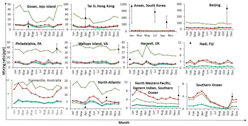
| dxdt=f(t,x), | (5) |
| dydt=g(y). | (6) |
(5) is called asymptotically autonomous with limit equation (6) if
| f(t,x)→g(x),t→∞, locally uniformly in x∈Rn, |
i.e., for
Lemma 3.2 ([23]). The
| dist(x(t),Ω)→0,t→∞. |
Finally
Lemma 3.3 ([23]). Let
Now, consider the following sub-model of (1)
| {dSdt=A+δV−λSI−mS−θS,dIdt=λSI−mI−kI,dVdt=θS−δV−mV. | (7) |
Lemma 3.4. For system (7), we have the following claims:
(1) If
(2) If
Proof. (1) Consider a Lyapunov function defined by
| L(S,I,V)=(S−S0−S0lnSS0)+(V−V0−V0lnVV0)+I. |
Differentiating
| dLdt=(1−S0S)dSdt+(1−V0V)dVdt+dIdt=(m+k)(R0−1)I+A(2−SS0−S0S)+δV0(1+VV0−SS0−S0VSV0)+θS0(1+SS0−VV0−SV0S0V)=(m+k)(R0−1)I+mS0(2−SS0−S0S)+θS0(2−SS0−S0S)−δV0(2−SS0−S0S)+θS0(1+SS0−VV0−SV0S0V)−δV0(1+SS0−VV0−SV0S0V)+δV0(1+SS0−VV0−SV0S0V)+δV0(1+VV0−SS0−S0VSV0)=(m+k)(R0−1)I+mS0(2−SS0−S0S)+mV0(3−S0S−VV0−SV0S0V)+δV0(2−SV0S0V−S0VSV0). |
If
(2) Consider the Lyapunov function
| L(S,I,V)=S−S∗−S∗lnSS∗+I−I∗−I∗lnII∗+V−V∗−V∗lnVV∗. |
Differentiating
| dLdt=(1−S∗S)(A+δV−λSI−mS−θS)+(1−I∗I)(λSI−mI−kI)+(1−V∗V)(θS−δV−mV)=A(2−S∗S−SS∗)+δV∗(SS∗−1)(S∗VSV∗−1)+θS∗(VV∗−1)(SV∗S∗V−1)=2A+δV∗+θS∗−SS∗(mS∗+λS∗I∗)−mV−AS∗S−δVS∗S−θSV∗V=(λS∗I∗+mS∗)(2−S∗S−SS∗)+δV∗(2−S∗VSV∗−SV∗S∗V)+3mV∗(3−S∗S−VV∗−SV∗S∗V)≤0. |
Obviously,
Theorem 3.5. For system (1), we have the following conclusions:
(1) If
(2) If
Proof.
Now, consider the rest equations of (1) except (7), that is,
| {dS1dt=Λ1+(1−q1)γ1I1−βS1I(t)−d1S1,dI1dt=βS1I(t)−γ1I1−d1I1,dC1dt=q1γ1I1−d1C1dS2dt=Λ2+(1−q2)γ2I2−εβS2I(t)−d2S2,dI2dt=εβS2I(t)−γ2I2−d2I2,dC2dt=q2γ2I2−d2C2. | (8) |
When
| {dS1dt=Λ1+(1−q1)γ1I1−d1S1,dI1dt=−γ1I1−d1I1,dC1dt=q1γ1I1−d1C1,dS2dt=Λ2+(1−q2)γ2I2−d2S2,dI2dt=−γ2I2−d2I2,dC2dt=q2γ2I2−d2C2. | (9) |
Obviously, the linear system (9) admits a unique equilibrium
(2) When
| {dS1dt=Λ1+(1−q1)γ1I1−βS1I∗−d1S1,dI1dt=βS1I∗−γ1I1−d1I1,dC1dt=q1γ1I1−d1C1dS2dt=Λ2+(1−q2)γ2I2−εβS2I∗−d2S2,dI2dt=εβS2I∗−γ2I2−d2I2,dC2dt=q2γ2I2−d2C2. | (10) |
It is not difficult to show that the linear system (10) has an equilibrium
The brucellosis asserts heavy burden to human health and local economy. The government consequently has to adopt a series of measures to control the brucellosis. In theory, by the global threshold dynamics of (1), from the explicit expressions of
In reality, the financial support from the government is very limited and can not meet the real requirement of the brucellosis control. The testing of sheep brucella and the culling of infected sheep can not be sustainedly and effectively implemented in large scale[41]. Some moderate measures have been carried out to control the brucellosis such as vaccination program in sheep stock and health education in human population aiming to raise the consciousness among publics to protect against brucellosis by influencing self examination behavior.
Taking into account the serious situation of the brucellosis in Inner Mongolia and the limited financial support from the government, one has to find a balance between the loss induced by brucellosis and the cost of control effort. It is very important and reasonable to achieve the best control effect with given limited financial budget.
Optimization has been playing a key role in the design, planning and operation of infectious disease control and related processes. It is reasonable and challenging to develop optimal strategy for more effective control or treatment options of infectious diseases in resource-limited settings. Brucellosis infections and their control are a world-wide challenge due to limited available resources.
In the following, we explore the optimal control strategy for brucellosis by considering both the control effectiveness and resource limitation. According to the reality of brucellosis control in Inner Mongolia, we still take vaccination in sheep stock and health education in human population as control measures in our optimal control model. Then the vaccination rate
| U={(θ(t),φ1(t),φ2(t))|0≤θ(t)≤ˉθ, 0≤φi(t)≤¯φi, 0≤t≤T, θ(t)and φi(t)are Lebesgue measurable,i=1,2}. | (11) |
In most real-life optimization scenarios and designs of the control of brucellosis, multiple objectives under consideration arise naturally and often conflict with each other. Anyone actually prefers to achieve best control by using less effort or cost, i.e., minimize cost, maximize performance, maximize reliability, etc. It seems very difficult but realistic.
Here our key objectives are to minimize the cost for vaccination and health education and to minimize the economic loss caused by culling of infected sheep and treatment of infected human cases. These costs during
| ∫T0B0S(t)θ(t)dt,∫T02∑i=1BiSi(t)φi(t)dt,∫T0D0kI(t)dt,∫T0(D1(I1(t)+I2(t))+D2(C1(t)+C2(t)))dt, | (12) |
respectively, where
Now, we are facing with a multi-objective optimization problem
| min∫T0D0kI(t)dt,min∫T0(D1(I1(t)+I2(t))+D2(C1(t)+C2(t)))dt,min∫T0B0S(t)θ(t)dt,min∫T02∑i=1BiSi(t)φi(t)dt, | (13) |
subject to
| dSdt=A+δV−λSI−mS−θ(t)S,dIdt=λSI−mI−kI,dVdt=θ(t)S−δV−mV,dS1dt=Λ1+(1−q1)γ1I1−β(1−φ1(t))S1I−d1S1,dI1dt=β(1−φ1(t))S1I−γ1I1−d1I1,dC1dt=q1γ1I1−d1C1,dS2dt=Λ2+(1−q2)γ2I2−εβ(1−φ2(t))S2I−d2S2,dI2dt=εβ(1−φ2(t))S2I−γ2I2−d2I2,dC2dt=q2γ2I2−d2C2,(θ(t),φ1(t),φ2(t))∈U, | (14) |
with initial conditions
| 0≤S(0)≤M,0≤I(0)≤M,0≤V(0)≤M,0≤Si(0)≤M,0≤Ii(0)≤M,0≤Ci(0)≤M, i=1,2, | (15) |
where
In term of methodology, there are several different approaches to solve general continuous multi-objective optimization problems[24]. One of the most common approaches is in general known as the weighted sum or scalarization method, which minimizes a positively weighted convex sum of the objectives by combining its multiple objectives into one single-objective scalar composite function with equal or weighted treatment.
By the weighted sum method, we transformed the vector-valued optimization problem (13)-(15) into a scalar quadratic optimization problem with a unique objective function of the following form
| J(θ(t),φ1(t),φ2(t))=∫T0[ω1(D0kI(t))2+ω2((D1(I1(t)+I2(t)))2+(D2(C1(t)+C2(t)))2)+ω3(B0S(t)θ(t))2+ω4∑2i=1(BiSi(t)φi(t))2]dt, | (16) |
subjected to (14), (15), and
To facilitate the discussions below, let
| min(θ(t),φ1(t),φ2(t))∈UJ(θ(t),φ1(t),φ2(t)), | (17) |
subject to
| dXdt=F(t,X,u), X(0)≥0, | (18) |
where
In the optimal control theory, after formulating the model and the corresponding objective functionals appropriate to the scenarios, one has to explore several basic problems such as proving the existence of an optimal control and characterizing the optimal control. In order to prove the existence of an optimal control, we introduce the following conclusion ([12], Theorem 4.1 and Corollary 4.1).
Lemma 4.1. Consider the optimal control problem
| minu∈DJ(u)=minu∈D∫t1t0L(t,x,u)dt+ϕ(e) |
subject to
Theorem 4.2. There exists an optimal pair
| J(θ∗(t),φ∗1(t),φ∗2(t))=min(θ,φ1,φ2)∈UJ(θ(t),φ1(t),φ2(t)) |
subject to (18), where
Proof. It suffices to show that the conditions of Lemma 4.1 are satisfied with
The claim
Let
| Φ(t,X,v)≥C1(|θ|2+|φ1|2+|φ2|2)γ2−C2 |
since
In order to verify
| U+={(n,m)|∃v∈U,m=F(t,X,v), n≥Φ(t,X,v)}. |
For any
| m1=F(t,X,v1), n1≥Φ(t,X,v1),m2=F(t,X,v2), n2≥Φ(t,X,v2). |
Since
| sm1+(1−s)m2=sF(t,X,v1)+(1−s)F(t,X,v2)=F(t,X,sv1+(1−s)v2). |
Note that the control set
| sm1+(1−s)m2=F(t,X,sv1+(1−s)v2)=F(t,X,u) |
for
| sn1+(1−s)n2≥sΦ(t,X,v1)+(1−s)Φ(t,X,v2)≥Φ(t,X,sv1+(1−s)v2)=Φ(t,X,u). |
Then, for
Next, we characterize the optimal control by deriving necessary conditions for the optimal control with the help of Pontryagin's Maximum Principle.
Theorem 4.3. The optimal control of (17) is characterized by
| θ∗(t)=min{ˉθ,max{λ1−λ32ω3B20S∗(t),0}},φ∗1(t)=min{¯φ1,max{(λ5−λ4)βI∗(t)2ω4B21S∗1(t),0}},φ∗2(t)=min{¯φ2,max{(λ8−λ7)εβI∗(t)2ω4B22S∗2(t),0}}, | (19) |
where
Proof. In order to facilitate the discussion below, we kill the stars in the optimal state
By Pontryagin's Maximum Principle, as in [7,28,31], to find the optimal control of (17)-(18) is equivalent to minimize the following Hamiltonian
| H=ω1(D0kI(t))2+ω2((D1(I1(t)+I2(t)))2+(D2(C1(t)+C2(t)))2)+ω3(B0S(t)θ(t))2+ω42∑i=1(BiSi(t)φi(t))2+9∑i=1λifi, |
where
| λ′1=−∂H∂S=−2ω3B20θ2(t)S(t)+λ1λI+λ1m+λ1θ(t)−λ2λI−λ3θ(t),λ′2=−∂H∂I=−2ω1D20k2I(t)+λ1λS−λ2(λS−m−k)+λ4β(1−φ1(t))S1−λ5β(1−φ1(t))S1+λ7εβ(1−φ2(t))S2−λ8εβ(1−φ2(t))S2,λ′3=−∂H∂V=−λ1δ+λ3(δ+m),λ′4=−∂H∂S1=−2ω4B21φ21(t)S1(t)+λ4(β(1−φ1(t))I+d1)−λ5β(1−φ1(t))I,λ′5=−∂H∂I1=−2ω2D21(I1(t)+I2(t))−λ4(1−q1)γ1+λ5(γ1+d1)−λ6q1γ1,λ′6=−∂H∂C1=−2ω2D22(C1(t)+C2(t))+λ6d1,λ′7=−∂H∂S2=−2ω4B22φ22(t)S2(t)+λ7(εβ(1−φ2(t))I+d2)−λ8εβ(1−φ2(t))I,λ′8=−∂H∂I2=−2ω2D21(I1(t)+I2(t))−λ7(1−q2)γ2+λ8(γ2+d2)−λ9q2γ2,λ′9=−∂H∂C2=−2ω2D22(C1(t)+C2(t))+λ9d2 | (20) |
and the transversality conditions
| λi(T)=0, i=1,2,...,9. | (21) |
The optimality conditions
| ∂H∂θ(t)|(θ∗,φ∗1(t),φ∗2(t))=0, ∂H∂φi(t)|(θ∗,φ∗1(t),φ∗2(t))=0 |
lead to
| θ∗(t)=λ1−λ32ω3B20S∗(t), φ∗1(t)=(λ5−λ4)βI∗(t)2ω4B21S∗1(t), φ∗2(t)=(λ8−λ7)εβI∗(t)2ω4B22S∗2(t). |
Moreover, taking into account the fact that
In this section, we first use (1) to simulate the reported sheep brucellosis and human brucellosis data of Inner Mongolia from 2001 to 2010 and to predict the trends of the brucellosis. Then, we perform sensitivity analysis of some key parameters, numerically simulate the optimal control, and seek for some effective control and prevention measures.
The data of sheep population is extracted from China Animal Husbandry Yearbook [8] (see Table 2). The data, concerning human brucellosis from 2001 to 2014, are adopted from China Health Statistics Yearbook[25] (see Table 3). The data of sheep brucellosis can not be acquired easily since there are few published studies on the population dynamics of sheep, and we calculate the number of brucellosis sheep in Inner Mongolia (see Table 2) from data of sheep population in Table 2 and the annual seroprevalence of sheep brucella in key monitoring regions of Inner Mongolia[11,13,22,30,38,39,43].
| Year | 2001 | 2002 | 2003 | 2004 | 2005 |
| Sheep Breeding[8] | 3551.6 | 3515.9 | 3951.7 | 4450.6 | 5318.48 |
| Sale and Slaughter[8] | 2081.2 | 2146.5 | 2156 | 2867.74 | 3782.99 |
| Brucellosis sheep1 | 33.74 | 35.15 | 59.27 | 89.1 | 132.95 |
| Year | 2006 | 2007 | 2008 | 2009 | 2010 |
| Sheep Breeding[8] | 5419.99 | 5594.44 | 5063.29 | 5125.3 | 5197.2 |
| Sale and Slaughter[8] | 4539.6 | 5011.05 | 4874.94 | 5183.7 | 5339.2 |
| Brucellosis sheep1 | 162.57 | 195.79 | 202.52 | 230.63 | 259.85 |
| 1 Calculated from data of sheep breeding and the annual seroprevalence of sheep brucella in key monitoring regions of Inner Mongolia[11,13,22,30,38,39,43]. | |||||
DownLoad: CSV| Year | 2001 | 2002 | 2003 | 2004 | 2005 | 2006 | 2007 |
| Reported Human Cases | 420 | 610 | 1280 | 4140 | 8740 | 8050 | 8117 |
| Year | 2008 | 2009 | 2010 | 2011 | 2012 | 2013 | 2014 |
| Reported Human Cases | 11105 | 16551 | 16935 | 20845 | 12817 | 9310 | 10538 |
DownLoad: CSVIn Inner Mongolia, the total population was about 24 million in the past decade with the birth rate less than
In order to carry out numerical simulations, most parameters of (1) are obtained from literature or assumed on the basis of common sense(see Table 1). The transmission rates of brucellosis (i.e.,
 Figure 2. Predicted tendency of brucellosis in Inner Mongolia. The solid line represents the prediction of (1) and the diamonds are the reported data in Inner Mongolia of P. R. China. (a) Number of brucellosis sheep (
With the help of (1), we fit it with the data from 2001 to 2011 and predict the dynamics of both sheep brucellosis infection and human brucellosis infection in Inner Mongolia (Fig. 2). The numerical simulations show that the model (1) with reasonable parameter values provides a good match to the reported data. From 2001 to 2011, the brucellosis sheep and human brucellosis cases kept increasing. From 2012 to 2015, due to the government's strong intervention on the transmission of brucellosis (e.g., a special fund was set to cull the infected sheep) [17,35,40], the size of brucellosis sheep and human brucellosis cases had a significant decline. However, the epidemic situation will become more serious in the coming decades and reach a peak at about 2040 if the government of Inner Mongolia can not sustainedly provide enough support to cull the infected sheep (see Fig. 2).
In order to better understand the mechanism and the control of brucellosis, we characterize the influence of some key parameters or factors in (1) by sensitivity analysis. Fig. 3-6 provide sensitivity analysis for (1) in terms of
 Figure 3. Influence of vaccination (
 Figure 4. Influence of the recruitment of sheep (
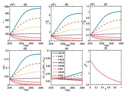 Figure 5. Influence of culling of the infected sheep (
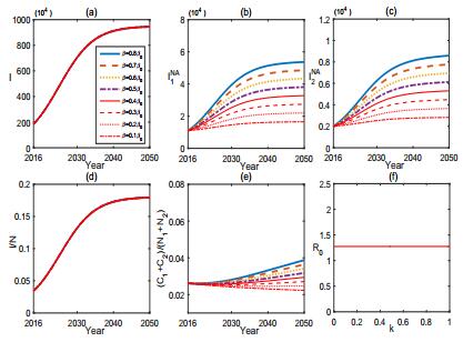 Figure 6. Influence of the transmission rate between brucellosis sheep and human(
From Fig. 3, we find that the vaccination of sheep can effectively control the brucellosis in some extent but can not eradicate it from either the sheep or human. Fig. 4 shows the sensitivity of (1) to
Culling the infected sheep is another effective measure to control the brucellosis. Fig. 5 depicts that increasing the culling rate
According to the above sensitivity analysis and numerical experiments, by comparing those figures, the recruitment of susceptible sheep and the culling of infected sheep are more sensitive than vaccination and health education in the current brucellosis outbreak in Inner Mongolia. In conclusion, controlling the population of sheep, reducing the birth rate of sheep, increasing the vaccination rate of sheep, improving the culling management of infected sheep, enhancing the people's awareness of brucellosis, and any combination of these measures are effective to control brucellosis. In practice, some policy involving comprehensive measures must be brought into operation.
By Forward-Backward sweep method [21], we further expound the optimal control by numerical experiments. According to the current economic status in Inner Mongolia, the cost of culling each infected sheep is about 1000 CNY (
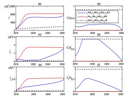 Figure 7. The optimal control
 The optimal control strategy explored in Section 4 sensitively depends on the selection of weighted coefficients. Since the principal aim is to reduce the number of brucellosis human and sheep cases, it is reasonable to assume that both
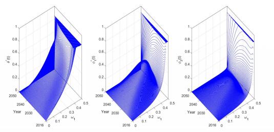 Figure 8. Simulation of the optimal control
 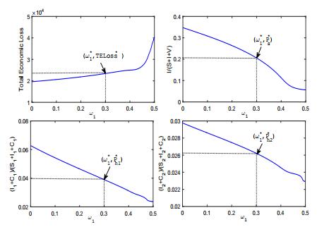 Figure 9. Total economic loss (i.e., the sum of the four integrals in (12)) and prevalence rates vary with the weighted coefficients. The policy-maker should confirm the weight coefficients according to the financial budget for brucellosis (
Simulations in Fig. 10-11 reveal that the culling of infected sheep and the recruitment of sheep play important roles on the optimal control of brucellosis. Fig. 10 shows that, when the culling rate
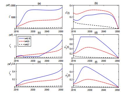 Figure 10. Simulations of the optimal control
 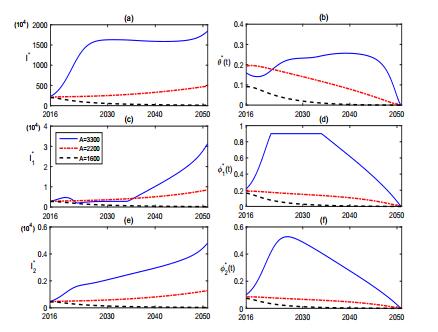 Figure 11. Simulations of the optimal control
 The transmission of brucellosis has been a growing public concern in China, particularly in Inner Mongolia. In this study, we formulate a multigroup epidemiological model to study the transmission dynamics and explore control strategies for the brucellosis in Inner Mongolia. Our theoretical and numerical findings indicate that the brucellosis gradually increases in the next decades and reaches a peak at about 2030. Vaccination and health-prevention education, which are the main currently working control measures, positively affect and facilitate the disease control (see Fig. 3 and Fig. 6), but can not eliminate the brucellosis in Inner Mongolia (see Fig. 7). Sensitivity analyses in Fig. 4 and Fig. 5 show that the population size of sheep and the culling rate of brucellosis sheep are two important factors triggering the serious epidemic situation. The brucellosis in both sheep and human can be well controlled when the breeding size of sheep is reduced or the culling rate of infectious sheep is enhanced. Fig. 10 and Fig. 11 provide a series of effective and time-variable control strategies when the culling rate of brucellosis sheep is increased and when the population size of sheep is decreased, respectively. The numerical solutions of the optimal controls illustrated in Fig. 10 and Fig. 11 provides practical guidance for policymakers to make effective control policy and to implement it in resources-limited setting.
The study reveals that the brucellosis in Inner Mongolia of China is hardly eliminated if the policymakers still pay most attentions to the vaccination in sheep stock and the health-prevention education in human population. Our studies suggest that the government and the policymakers must take a new look at the current working control strategies. A reasonable and effective control strategy must involve comprehensive control measures based on the optimal control study.
Finally, we would like to point out that, even if a costly policy can prevent the disease spread, the prevention policy might not be well executed in resource-limited setting. A fundamental challenge in many control problems in epidemics is to find the right balance amongst several objectives. Although the weighted sum method is a typical method or technique to solve the multi-objective optimization, the problem lies in the correct selection of the weights to characterize the decision-makers preferences. In practice, it can be very difficult to precisely and accurately select these weights, even for someone very familiar with the problem domain. In addition, perturbations in the weights can lead to different solutions (see (19)). For this reason and others, decision-makers often prefer a set of promising solutions given the multiple objectives. In addition, recently, some evolutionary approaches have been proposed to deal with multi-objective optimization problems. Genetic algorithms, being a population based approach, is a well suited heuristic approach, see[18] for an overview and tutorial of multiple-objective optimization methods using genetic algorithms (GA). It is interesting but challenging to investigate the optimal control problem in this study by GA and compare it with the weighted sum method. It is left for our future work.
This work is partially supported by the National Natural Science Foundation of P. R. China (No. 11671072,11271065,11426045), the Research Fund for the Doctoral Program of Higher Education of P. R. China (No.20130043110001), and the Research Fund for Chair Professors of Changbai Mountain Scholars Program.
| [1] |
Wine PH, Chameides WL, Ravishankara AR (1981) Potential role of CS2 photooxidation in tropospheric sulfur chemistry. Geophys Res Lett 8: 543-546. doi: 10.1029/GL008i005p00543

|
| [2] |
Andreae MO (1990) Ocean-atmosphere interactions in the global biogeochemical sulfur cycle. Mar Chem 30: 1-29. doi: 10.1016/0304-4203(90)90059-L
|
| [3] |
Khalil MAK, Rasmussen RA (1984) Global sources, lifetimes and mass balances of carbonyl sulphide (OCS) and carbon disulfide (CS2) in the Earth's atmosphere. Atmos Environ 18: 1805-1813. doi: 10.1016/0004-6981(84)90356-1
|
| [4] |
Leck C, Rodhe H (1991) Emissions of marine biogenic sulfur to the atmosphere of northern Europe. J Atmos Chem 12: 63-86. doi: 10.1007/BF00053934
|
| [5] |
Kim K-H, Andreae MO (1992) Carbon disulfide in the estuarine, coastal, and oceanic environments. Marine Chem 40: 179-197. doi: 10.1016/0304-4203(92)90022-3
|
| [6] |
Xie H, Moore RM, Miller WL (1998) Photochemical production of carbon disulphide in seawater. J Geophys Res 103: 5635-5644. doi: 10.1029/97JC02885
|
| [7] |
Xie H, Moore RM, Miller WL (1999) Carbon disulfide in the North Atlantic and Pacific oceans. J Geophys Res 104: 5393-5402. doi: 10.1029/1998JC900074
|
| [8] |
Kettle AJ, Rhee TS, von Hobe M, et al. (2001) Assessing the flux of different volatile sulfur gases from the ocean to the atmosphere. J Geophys Res 106: 12193-12209. doi: 10.1029/2000JD900630
|
| [9] |
Chin M, Davis DD (1993) Global sources and sinks of OCS and CS2 and their distributions. Global Biogeochem. Cycles 7: 321-337. doi: 10.1029/93GB00568
|
| [10] | Watts SF (2000) The mass budgets of carbonyl sufide, dimethyl sulphide, carbon disulfide and hydrogen sulphide. Atmos Environ 34: 761-779. |
| [11] | Blake NJ, Streets DG, Woo JH, et al. (2004) Carbonyl sulphide and carbon disulfide: large-scale distributions over the western Pacific and emissions from Asia during TRACE-P. J Geophys Res 109: D15. |
| [12] | Ren YL (1999) Is carbonyl sulfide a precursor for carbon disulfide in vegetation and soil? Interconversion of carbonyl sulfide and carbon disulfide in fresh grain tissues in vitro. J Agric Food Chem 47: 2141-2144. |
| [13] |
Steinbacher M, Bingemer HG, Schmidt U (2004) Measurements of the exchange of carbonyl sulfide (OCS) and carbon disulfide (CS2) between soil and atmosphere in a spruce forest in central Germany. Atmos Environ 38: 6043-6052. doi: 10.1016/j.atmosenv.2004.06.022
|
| [14] |
Stickel RE, Chin M, Daykin EP, et al. (1993). Mechanistic studies of the OH-initiated oxidation of CS2 in the presence of O2. J Phys Chem 97: 13653-13661. doi: 10.1021/j100153a038
|
| [15] | Seinfeld JH, Pandis SN (2006) Atmospheric Chemistry and Physics: From Air Pollution to Climate Change, 2 Eds., John Wiley and Sons, Inc., New Jersey: 1-1203. |
| [16] |
Crutzen PJ (1976) The possible importance of CSO for the sulfate layer of the stratosphere. Geophys Res Lett 3: 73-76. doi: 10.1029/GL003i002p00073
|
| [17] |
Hofmann DJ (1990) Increase in the stratospheric background sulfuric acid aerosol mass in the past 10 years. Science 248: 996-1000. doi: 10.1126/science.248.4958.996
|
| [18] | Taubman SJ, Kasting JF (1995). Carbonyl sufide: No remedy for global warming. Geophys Res Lett 22: 803-805. |
| [19] |
Chin M, Davis DD (1995) A reanalysis of carbonyl sulphide as a source of stratospheric background sulfur aerosol. J Geophys Res Atmos 100: 8993-9005. doi: 10.1029/95JD00275
|
| [20] | Bruhl C, Lelieveld J, Tost H, et al. (2015). Stratospheric sulfur and its implications for radiative forcing simulated by the chemistry climate model EMAC. J Geophys Res-Atmos 120: 2103-2118. |
| [21] | Xu X, Bingemer HG, Schmidt U (2002) The flux of carbonyl sulphide and carbon disulfide between the atmosphere and a spruce forest. Atmos Chem Phys 2: 171-181. |
| [22] | Taylor Jr GE, McLaughlin Jr SB, Shriner DS, et al. (1983). The flux sulfur-containing gases to vegetation. Atmos Environ 17: 789-796. |
| [23] |
De Bruyn WL, Swartz E, Hu JH, et al. (1995) Henry's law solubilities and setchenow coefficients for biogenic reduced sulfur species obtained from gas-liquid uptake measurements. J Geophys Res 100: 7245-7251. doi: 10.1029/95JD00217
|
| [24] |
Berglen TF, Berntsen TK, Isaksen SA, et al. (2004) A global model of the coupled sulphur/oxidant chemistry in the troposphere: The sulphur cycle. J Geophys Res 109: D19310. doi: 10.1029/2003JD003948
|
| [25] |
Kloster S, Feichter J, Maier-Reimer E, et al. (2006) DMS cycle in the marine ocean-atmosphere system- a global model study. Biogeosciences 3: 29-51. doi: 10.5194/bg-3-29-2006
|
| [26] | Kettle AJ, Kuhn U, Von Hobe M, et al. (2002) Global budget of atmospheric carbonyl sulfide: Temporal and spatial variations of the dominant sources and sinks. J Geophys Res 107: D22. |
| [27] |
Suntharalingam P, Kettle AJ, Monzka SM, et al. (2008) Global 3-D model analysis of the seasonal cycle of atmospheric carbonyl sulfide: Implications for terrestrial vegetation uptake. Geophys Res Lett 35: L19801. doi: 10.1029/2008GL034332
|
| [28] |
Berry J, Wolf A, Campbell JE, et al. (2013) A coupled model of the global cycles of carbonyl sulfide and CO2: A possible new window on the carbon cycle. J Geophys Res-Biogeo 118: 842-852. doi: 10.1002/jgrg.20068
|
| [29] | Kuai L, Worden JR, Campbell JE, et al. (2015) Estimate of carbonyl sulfide tropical oceanic surface fluxes using Aura Tropospheric Emission Spectrometer observations. J Geophys Res-Atmos 120: 11012-11023. |
| [30] |
Glatthor N, Höpfner M, Baker IT, et al. (2015) Tropical sources and sinks of carbonyl sulfide observed from space. Geophys Res Lett 42: 10082-10090. doi: 10.1002/2015GL066293
|
| [31] | Kremser S, Thomason LW, von Hobe M, et al. (2016) Stratospheric aerosol-Observations, processes, and impact on climate. Rev Geophys 54: 278-335. |
| [32] | Lennartz ST, Marandino CA, von Hobe M, et al. (2017) Direct oceanic emissions unlikely to account for the missing source of atmospheric carbonyl sulfide. Atmos Chem Phys 17: 385-402. |
| [33] | Pham M, Müller J-F, Brasseur GP, et al. (1995) A three-dimensional study of the tropospheric sulfur cycle. J Geophys Res 100: 26061-26092. |
| [34] |
Weisenstein DK, Yue GK, Ko MKW, et al. (1997) A two-dimensional model of sulfur species and aerosols. J Geophys Res 102: 13019-13035. doi: 10.1029/97JD00901
|
| [35] |
Kjellström E (1998) A three-dimensional global model study of carbonyl sulphide in the troposphere and the lower stratosphere. J Atmos Chem 29: 151-177. doi: 10.1023/A:1005976511096
|
| [36] | Stevenson DS, Collins WJ, Johnson CE, et al. (1998) Intercomparison and evaluation of atmospheric transport in a Lagrangian model (STOCHEM), and an Eulerian model (UM), using 222Rn as a short-lived tracer. Quat J Royal Meteorol Soc 124: 2477-3492. |
| [37] | Stevenson DS, Dentener FJ, Schultz MG, et al. (2006) Multimodel ensemble simulations of present-day and near-future tropospheric ozone. J Geophys Res 111: D08301. |
| [38] | Collins WJ, Stevenson DS, Johnson CE, et al. (1997) Tropospheric ozone in a Global-Scale Three-Dimensional Lagrangian Model and its response to NOx emission controls. J Atmos Chem 26: 223-274. |
| [39] | Utembe SR, Cooke MC, Archibald AT, et al. (2010) Using a reduced Common Representative Intermediates (CRI v2-R5) mechanism to simulate tropospheric ozone in a 3-D Lagrangian chemistry transport model. Atmos Environ 13: 1609-1622. |
| [40] |
Derwent RG, Collins WJ, Jenkin ME, et al. (2003) The global distribution of secondary particulate matter in a 3-D Lagrangian chemistry transport model. J Atmos Chem 44: 57-95. doi: 10.1023/A:1022139814102
|
| [41] | Stevenson DS, Johnson CE, Highwood EJ, et al. (2003) Atmospheric impact of the 1783–1784 Laki eruption: Part I chemistry modelling. Atmos Chem Phys 3: 487-507. |
| [42] | Derwent RG, Stevenson DS, Doherty RM, et al. (2008) How is surface ozone in Europe linked to Asian and North American NOx emissions? Atmos Environ 42: 7412-7422. |
| [43] | Jenkin ME, Watson LA, Utembe SR, et al. (2008) A Common Representative Intermediate (CRI) mechanism for VOC degradation. Part-1: gas phase mechanism development. Atmos Environ 42: 7185-7195. |
| [44] | Watson LA, Shallcross DE, Utembe SR, et al. (2008) A Common Representative Intermediate (CRI) mechanism for VOC degradation. Part 2: gas phase mechanism reduction. Atmos Environ 42: 7196-7204. |
| [45] | Utembe SR, Watson LA, Shallcross DE, et al. (2009) A Common Representative Intermediates (CRI) mechanism for VOC degradation. Part 3: Development of a secondary organic aerosol module. Atmos Environ 43: 1982-1990. |
| [46] |
Utembe SR, Cooke MC, Archibald AT, et al. (2011) Simulating secondary organic aerosol in a 3-D Lagrangian chemistry transport model using the reduced Common Representative Intermediates mechansim (CRI v2-R5). Atmos Environ 45: 1604-1614. doi: 10.1016/j.atmosenv.2010.11.046
|
| [47] |
Collins WJ, Stevenson DS, Johnson CE, et al. (2000) The European regional ozone distribution and its links with the global scale for the years 1992 and 2015. Atmos Environ 34: 255-267. doi: 10.1016/S1352-2310(99)00226-5
|
| [48] | Olivier JG, Bouwman AF, Berdowski JJ, et al. (1996) Description of EDGAR Version 2.0: A set of global emission inventories of greenhouse gases and ozone-depleting substances for all anthropogenic and most natural sources on a per country basis and on 1 degree ´ 1 degree grid. Technical report, Netherlands Environmental Assessment Agency. |
| [49] | Olivier JGJ, Berdowski JJM (2001) Global emissions sources and sinks. Berdowski JJM, Guicherit R, Heij BJ (Eds.). The Climate System, Swets and Zeitlinger Publishers, Lisse, Netherlands. |
| [50] | Granier C, Lamarque JF, Mieville A, et al. (2005) POET, a database of surface emissions of ozone precursors. Available from: http://accent.aero.jussieu.fr/database_table_inventories.php. |
| [51] |
Atkinson R, Baulch DL, Cox RA, et al. (2004) Evaluated kinetic and photochemical data for atmospheric chemistry: Volume I-gas phase reactions of Ox, HOx, NOx and SOx species. Atmos Chem Phys 4: 1461-1738. doi: 10.5194/acp-4-1461-2004
|
| [52] | Khan MAH, Cooke MC, Utembe SR, et al. (2015) A study of global atmospheric budget and distribution of acetone using global atmospheric model STOCHEM-CRI. Atmos Environ 112: 269-277. |
| [53] | Sander SP, Friedl RR, Golden DM, et al. (2006) Chemical kinetics and photochemical data for use in atmospheric studies. Evaluation number 15, JPL publication 06-2, Jet Propulsion Laboratory, Pasadena, CA. |
| [54] |
Lee CL, Brimblecombe P (2016) Anthropogenic contributions to global carbonyl sulfide, carbon disulfide and organosulfides fluxes. Earth-Sci Rev 160: 1-18. doi: 10.1016/j.earscirev.2016.06.005
|
| [55] | Majozi T, Veldhuizen P (2015) The chemicals industry in South Africa. American Inst. Chem. Eng (AlChE) July: 46-51. Available from: https://www.aiche.org/sites/default/files/cep/20150746.pdf |
| [56] |
Kim KH, Swan H, Shon ZH, et al. (2004) Monitoring of reduced sulfur compounds in the atmosphere of Gosan, Jeju Island during the Spring of 2001. Chemosphere 54: 515-526. doi: 10.1016/j.chemosphere.2003.07.003
|
| [57] | Guo H, Simpson IJ, Ding AJ, et al. (2010) Carbonyl sulphide, dimethyl sulphide and carbon disulfide in the Pearl River Delta of southern China: Impact of anthropogenic and biogenic sources. Atmos Environ 44: 3805-3813. |
| [58] |
Pal R, Kim KH, Jeon EC, et al. (2009) Reduced sulfur compounds in ambient air surrounding an industrial region in Korea. Environ Monit Assess 148: 109-125. doi: 10.1007/s10661-007-0143-z
|
| [59] | Yujing M, Hai W, Zhang X, et al. (2002) Impact of anthropogenic sources on carbonyl sulphide in Beijing City. J Geophys Res 107: D24. |
| [60] |
Maroulis PJ, Bandy AR (1980) Measurements of atmospheric concentrations of CS2 in the eastern United States. Geophys Res Letts 7: 681-684. doi: 10.1029/GL007i009p00681
|
| [61] |
Jones BMR, Cox RA, Penkett SA (1983) Atmospheric chemistry of carbon disulphide. J Atmos Chem 1: 65-86. doi: 10.1007/BF00113980
|
| [62] |
Thornton DC, Bandy AR (1993). Sulfur dioxide and dimethyl sulfide in the central pacific troposphere. J Atmos Chem 17: 1-13. doi: 10.1007/BF00699110
|
| [63] | Inomata Y, Hayashi M, Osada K, et al. (2006) Spatial distributions of volatile sulfur compounds in surface seawater and overlying atmosphere in the northwestern Pacific Ocean, eastern Indian Ocean, and Southern Ocean. Global Biogeochem Cycles 20: GB2022. |
| [64] |
Cooper DJ, Saltzman ES (1993) Measurements of atmospheric dimethylsulphide, hydrogen sulphide, and carbon disulfide during GTE/CITE 3. J Geophys Res 98: 23397-23409. doi: 10.1029/92JD00218
|
| [65] | Inomata Y, Iwasaka Y, Osada K, et al. (2006) Vertical distributions of particles and sulfur gases (volatile sulfur compounds and SO2) over East Asia: comparison with two aircraft-borne measurements under the Asian continental outflow in spring and winter. Atmos Environ 40: 430-444. |
| [66] |
Bandy AR, Thornton DC, Johnson JE (1993) Carbon disulfide measurements in the atmosphere of the western north Atlantic and the northwestern south Atlantic oceans. J Geophys Res-Atmos 98: 23449-23457. doi: 10.1029/93JD02411
|
| 1. | Xuhua Ran, Jiajia Cheng, Miaomiao Wang, Xiaohong Chen, Haoxian Wang, Yu Ge, Hongbo Ni, Xiao-Xuan Zhang, Xiaobo Wen, Brucellosis seroprevalence in dairy cattle in China during 2008–2018: A systematic review and meta-analysis, 2019, 189, 0001706X, 117, 10.1016/j.actatropica.2018.10.002 | |
| 2. | Cheng Peng, Hao Zhou, Peng Guan, Wei Wu, De‐Sheng Huang, An estimate of the incidence and quantitative risk assessment of human brucellosis in mainland China, 2020, 1865-1674, 10.1111/tbed.13518 | |
| 3. | Xuhua Ran, Xiaohong Chen, Miaomiao Wang, Jiajia Cheng, Hongbo Ni, Xiao-Xuan Zhang, Xiaobo Wen, Brucellosis seroprevalence in ovine and caprine flocks in China during 2000–2018: a systematic review and meta-analysis, 2018, 14, 1746-6148, 10.1186/s12917-018-1715-6 | |
| 4. | Gui-Quan Sun, Ming-Tao Li, Juan Zhang, Wei Zhang, Xin Pei, Zhen Jin, Transmission dynamics of brucellosis: Mathematical modelling and applications in China, 2020, 18, 20010370, 3843, 10.1016/j.csbj.2020.11.014 | |
| 5. | Abdullah M. Alkahtani, Mohammed M. Assiry, Harish C. Chandramoorthy, Ahmed M. Al-Hakami, Mohamed E. Hamid, Sero-prevalence and risk factors of brucellosis among suspected febrile patients attending a referral hospital in southern Saudi Arabia (2014–2018), 2020, 20, 1471-2334, 10.1186/s12879-020-4763-z | |
| 6. | Paride O. Lolika, Steady Mushayabasa, Dynamics and Stability Analysis of a Brucellosis Model with Two Discrete Delays, 2018, 2018, 1026-0226, 1, 10.1155/2018/6456107 | |
| 7. | Yun Lin, Minghan Xu, Xingyu Zhang, Tao Zhang, Abdallah M. Samy, An exploratory study of factors associated with human brucellosis in mainland China based on time-series-cross-section data from 2005 to 2016, 2019, 14, 1932-6203, e0208292, 10.1371/journal.pone.0208292 | |
| 8. | Yin Li, Dan Tan, Shuang Xue, Chaojian Shen, Huajie Ning, Chang Cai, Zengzai Liu, Prevalence, distribution and risk factors for brucellosis infection in goat farms in Ningxiang, China, 2021, 17, 1746-6148, 10.1186/s12917-021-02743-x | |
| 9. | PSEUDO ALMOST AUTOMORPHY OF TWO-TERM FRACTIONAL FUNCTIONAL DIFFERENTIAL EQUATIONS, 2018, 8, 2156-907X, 1604, 10.11948/2018.1604 | |
| 10. | Shu-yi Ma, Zhi-guo Liu, Xiong Zhu, Zhong-zhi Zhao, Zhi-wei Guo, Miao Wang, Bu-yun Cui, Jun-yan Li, Zhen-jun Li, Molecular epidemiology of Brucella abortus strains from cattle in Inner Mongolia, China, 2020, 183, 01675877, 105080, 10.1016/j.prevetmed.2020.105080 | |
| 11. | Cheng Peng, Yan-Jun Li, De-Sheng Huang, Peng Guan, Spatial-temporal distribution of human brucellosis in mainland China from 2004 to 2017 and an analysis of social and environmental factors, 2020, 25, 1342-078X, 10.1186/s12199-019-0839-z | |
| 12. | Di Li, Lifei Li, Jingbo Zhai, Lingzhan Wang, Bin Zhang, Epidemiological features of human brucellosis in Tongliao City, Inner Mongolia province, China: a cross-sectional study over an 11-year period (2007–2017), 2020, 10, 2044-6055, e031206, 10.1136/bmjopen-2019-031206 | |
| 13. | Peng Guan, Wei Wu, Desheng Huang, Trends of reported human brucellosis cases in mainland China from 2007 to 2017: an exponential smoothing time series analysis, 2018, 23, 1342-078X, 10.1186/s12199-018-0712-5 | |
| 14. | Zhiguo Liu, Dongyan Liu, Miao Wang, Zhenjun Li, Human brucellosis epidemiology in the pastoral area of Hulun Buir city, Inner Mongolia autonomous region, China, between 2003 and 2018, 2022, 69, 1865-1674, 1155, 10.1111/tbed.14075 | |
| 15. | Xiaoxiao Liu, Chunrui Zhang, Stability and Optimal Control of Tree-Insect Model under Forest Fire Disturbance, 2022, 10, 2227-7390, 2563, 10.3390/math10152563 | |
| 16. | Yupeng Fang, Jianjun Wang, Guanyin Zhang, Fengdong Zhu, Chaoyue Guo, Jiandong Zhang, Kaixuan Guo, Yun Deng, Jinxue Zhang, Huanchun Chen, Zhengfei Liu, Enzootic epidemiology of Brucella in livestock in central Gansu Province after the National Brucellosis Prevention and Control Plan, 2023, 3, 2731-0442, 10.1186/s44149-023-00077-9 | |
| 17. | Adison Thongtha, Chairat Modnak, The bison–human–environment dynamics of brucellosis infection with prevention and control studies, 2023, 2195-268X, 10.1007/s40435-023-01194-6 | |
| 18. | Lei-Shi Wang, Ming-Tao Li, Xin Pei, Juan Zhang, Gui-Quan Sun, Zhen Jin, Cost assessment of optimal control strategy for brucellosis dynamic model based on economic factors, 2023, 10075704, 107310, 10.1016/j.cnsns.2023.107310 | |
| 19. | 雨欣 王, Modeling of Brucellosis Dynamics and Its Control Measures Based on Price Factors, 2023, 12, 2324-7991, 2502, 10.12677/AAM.2023.125252 | |
| 20. | Wei Lv, Si-Ting Zhang, Lei Wang, Multi-objective optimal control of tungiasis diseases with terminal demands, 2024, 17, 1793-5245, 10.1142/S1793524523500262 | |
| 21. | Haitham Taha, Carl Smith, Jo Durham, Simon Reid, Identification of a One Health Intervention for Brucellosis in Jordan Using System Dynamics Modelling, 2023, 11, 2079-8954, 542, 10.3390/systems11110542 | |
| 22. | Xiaoxiao Liu, Chunrui Zhang, Forest model dynamics analysis and optimal control based on disease and fire interactions, 2024, 9, 2473-6988, 3174, 10.3934/math.2024154 | |
| 23. | Meng Zhang, Xinrui Chen, Qingqing Bu, Bo Tan, Tong Yang, Liyuan Qing, Yunna Wang, Dan Deng, Spatiotemporal dynamics and influencing factors of human brucellosis in Mainland China from 2005–2021, 2024, 24, 1471-2334, 10.1186/s12879-023-08858-w | |
| 24. | Xiaohui Wen, Yun Wang, Zhongjun Shao, The spatiotemporal trend of human brucellosis in China and driving factors using interpretability analysis, 2024, 14, 2045-2322, 10.1038/s41598-024-55034-4 | |
| 25. | Feng Chen, Jing Hu, Yuming Chen, Qimin Zhang, Stability of a stochastic brucellosis model with semi-Markovian switching and diffusion, 2024, 89, 0303-6812, 10.1007/s00285-024-02139-z | |
| 26. | Shuangjie Bai, Boqiang Cao, Ting Kang, Qingyun Wang, A two-stage sheep-environment coupled brucellosis transmission dynamic model: Stability analysis and optimal control, 2024, 0, 1531-3492, 0, 10.3934/dcdsb.2024126 | |
| 27. | Xin 鑫 Pei 裴, Xuan-Li 绚丽 Wu 武, Pei 沛 Pei 裴, Ming-Tao 明涛 Li 李, Juan 娟 Zhang 张, Xiu-Xiu 秀秀 Zhan 詹, Dynamic modeling and analysis of brucellosis on metapopulation network: Heilongjiang as cases, 2025, 34, 1674-1056, 018904, 10.1088/1674-1056/ad92ff | |
| 28. | Weihao Li, Hanqi Ouyang, Ziyu Zhao, Liying Wang, Weiwei Meng, Sanji Zhou, Guojing Yang, Trends and age-period-cohort effect on incidence of brucellosis from 2006 to 2020 in China, 2024, 260, 0001706X, 107475, 10.1016/j.actatropica.2024.107475 | |
| 29. | Liu Yang, Meng Fan, Youming Wang, Fedor Korennoy, Dynamic Modeling of Prevention and Control of Brucellosis in China: A Systematic Review, 2025, 2025, 1865-1674, 10.1155/tbed/1393722 | |
| 30. | Zhiguo Liu, Yue Shi, Chuizhao Xue, Min Yuan, Zhenjun Li, Canjun Zheng, Epidemiological and Spatiotemporal Clustering Analysis of Human Brucellosis — China, 2019−2023, 2025, 7, 2097-3101, 130, 10.46234/ccdcw2025.020 | |
| 31. | Sijia Liu, Jiajing Hu, Yifan Zhao, Xinyan Wang, Xuemei Wang, Prediction and control for the transmission of brucellosis in inner Mongolia, China, 2025, 15, 2045-2322, 10.1038/s41598-025-87959-9 | |
| 32. | Yuan Zhao, Dongfeng Pan, Yanfang Zhang, Lixu Ma, Hong Li, Jingjing Li, Shanghong Liu, Peifeng Liang, Spatial interpolation and spatiotemporal scanning analysis of human brucellosis in mainland China from 2012 to 2018, 2025, 15, 2045-2322, 10.1038/s41598-025-91769-4 | |
| 33. | Caihong Song, Zigen Song, Global dynamics and optimal control strategies for the brucellosis model with environmental saturation infection: An assessment of severely affected provinces in China, 2025, 03784754, 10.1016/j.matcom.2025.04.008 | |
| 34. | Huidi Chu, Xinmiao Rong, Liu Yang, Meng Fan, Dynamical analysis and optimal control strategy of seasonal brucellosis, 2025, 234, 03784754, 299, 10.1016/j.matcom.2025.03.003 | |
| 35. | Sadia Shihab Sinje, Md Kamrujjaman, Rubayyi T. Alqahtani, Forest beetle infestation and its impact on ecosystems: Effects of harvesting practices and fire disruptions, 2025, 10, 2473-6988, 9933, 10.3934/math.2025455 | |
| 36. | Liu Yang, Qi Wang, Youming Wang, Meng Fan, Establishment of Risk Classification Index for Animal Brucellosis by Stochastic Models, 2025, 00225193, 112187, 10.1016/j.jtbi.2025.112187 |
Figures(6) / Tables(3)

Anwar Khan, Benjamin Razis, Simon Gillespie, Carl Percival, Dudley Shallcross. Global analysis of carbon disulfide (CS2) using the 3-D chemistry transport model STOCHEM[J]. AIMS Environmental Science, 2017, 4(3): 484-501. doi: 10.3934/environsci.2017.3.484

| Parameter | Value/Range | Unit | Definition | Reference |
| 3300 | | Constant recruitment of sheep | [8] | |
| | 0.6 | year | Natural elimination or death rate of sheep | [8] |
| | [1, 3] | year | Mean effective period of vaccination | [9,33,42] |
| | | year | Culling rate of infectious sheep | [17,35,40,41] |
| | [0, 0.85] | year | Effective vaccination rate of susceptible sheep | [9,42,33] |
| | 12 | | Recruitment of | [27] |
| | 11 | | Recruitment of | [27] |
| | 0.006 | year | Natural death rate of human | [27] |
| | 0.25 | year | Acute onset period of human | [41] |
| | [0.32, 0.74] | year | Fraction of acute human cases turned into chronic cases | [41] |
| | | year | Transmission rate of sheep | Fitting |
| | | year | Transmission rate between sheep and | Fitting |
| | 0.17 | year | Infection risk attenuation coefficient of | Fitting |
| Note: |
||||
DownLoad: CSV| Year | 2001 | 2002 | 2003 | 2004 | 2005 |
| Sheep Breeding[8] | 3551.6 | 3515.9 | 3951.7 | 4450.6 | 5318.48 |
| Sale and Slaughter[8] | 2081.2 | 2146.5 | 2156 | 2867.74 | 3782.99 |
| Brucellosis sheep1 | 33.74 | 35.15 | 59.27 | 89.1 | 132.95 |
| Year | 2006 | 2007 | 2008 | 2009 | 2010 |
| Sheep Breeding[8] | 5419.99 | 5594.44 | 5063.29 | 5125.3 | 5197.2 |
| Sale and Slaughter[8] | 4539.6 | 5011.05 | 4874.94 | 5183.7 | 5339.2 |
| Brucellosis sheep1 | 162.57 | 195.79 | 202.52 | 230.63 | 259.85 |
| 1 Calculated from data of sheep breeding and the annual seroprevalence of sheep brucella in key monitoring regions of Inner Mongolia[11,13,22,30,38,39,43]. | |||||
DownLoad: CSV| Parameter | Value/Range | Unit | Definition | Reference |
| 3300 | | Constant recruitment of sheep | [8] | |
| | 0.6 | year | Natural elimination or death rate of sheep | [8] |
| | [1, 3] | year | Mean effective period of vaccination | [9,33,42] |
| | | year | Culling rate of infectious sheep | [17,35,40,41] |
| | [0, 0.85] | year | Effective vaccination rate of susceptible sheep | [9,42,33] |
| | 12 | | Recruitment of | [27] |
| | 11 | | Recruitment of | [27] |
| | 0.006 | year | Natural death rate of human | [27] |
| | 0.25 | year | Acute onset period of human | [41] |
| | [0.32, 0.74] | year | Fraction of acute human cases turned into chronic cases | [41] |
| | | year | Transmission rate of sheep | Fitting |
| | | year | Transmission rate between sheep and | Fitting |
| | 0.17 | year | Infection risk attenuation coefficient of | Fitting |
| Note: |
||||
| Year | 2001 | 2002 | 2003 | 2004 | 2005 |
| Sheep Breeding[8] | 3551.6 | 3515.9 | 3951.7 | 4450.6 | 5318.48 |
| Sale and Slaughter[8] | 2081.2 | 2146.5 | 2156 | 2867.74 | 3782.99 |
| Brucellosis sheep1 | 33.74 | 35.15 | 59.27 | 89.1 | 132.95 |
| Year | 2006 | 2007 | 2008 | 2009 | 2010 |
| Sheep Breeding[8] | 5419.99 | 5594.44 | 5063.29 | 5125.3 | 5197.2 |
| Sale and Slaughter[8] | 4539.6 | 5011.05 | 4874.94 | 5183.7 | 5339.2 |
| Brucellosis sheep1 | 162.57 | 195.79 | 202.52 | 230.63 | 259.85 |
| 1 Calculated from data of sheep breeding and the annual seroprevalence of sheep brucella in key monitoring regions of Inner Mongolia[11,13,22,30,38,39,43]. | |||||
| Year | 2001 | 2002 | 2003 | 2004 | 2005 | 2006 | 2007 |
| Reported Human Cases | 420 | 610 | 1280 | 4140 | 8740 | 8050 | 8117 |
| Year | 2008 | 2009 | 2010 | 2011 | 2012 | 2013 | 2014 |
| Reported Human Cases | 11105 | 16551 | 16935 | 20845 | 12817 | 9310 | 10538 |


