Perfusion-based co-culture model system for bone tissue engineering

Stephen W. Sawyer; Kairui Zhang; Jason A. Horton; Pranav Soman; Stephen W. Sawyer; Kairui Zhang; Jason A. Horton; Pranav Soman

doi:10.3934/bioeng.2020009

AIMS Bioengineering

2020, Volume 7, Issue 2: 91-105. doi: 10.3934/bioeng.2020009

Previous Article Next Article

Research article Special Issues

Perfusion-based co-culture model system for bone tissue engineering

1.
Department of Biomedical and Chemical Engineering, Syracuse University, Syracuse, NY, USA
2.
Department of Orthopedic Surgery, SUNY Upstate Medical University, Syracuse, NY, USA

Received: 07 May 2020 Accepted: 25 May 2020 Published: 29 May 2020

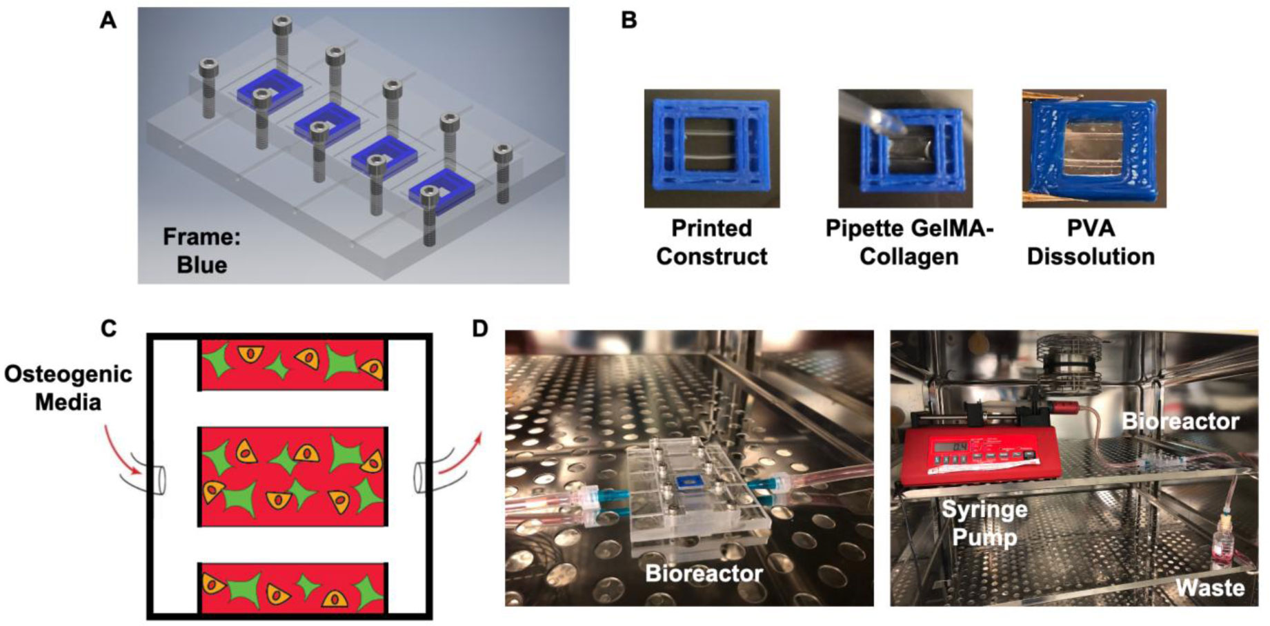
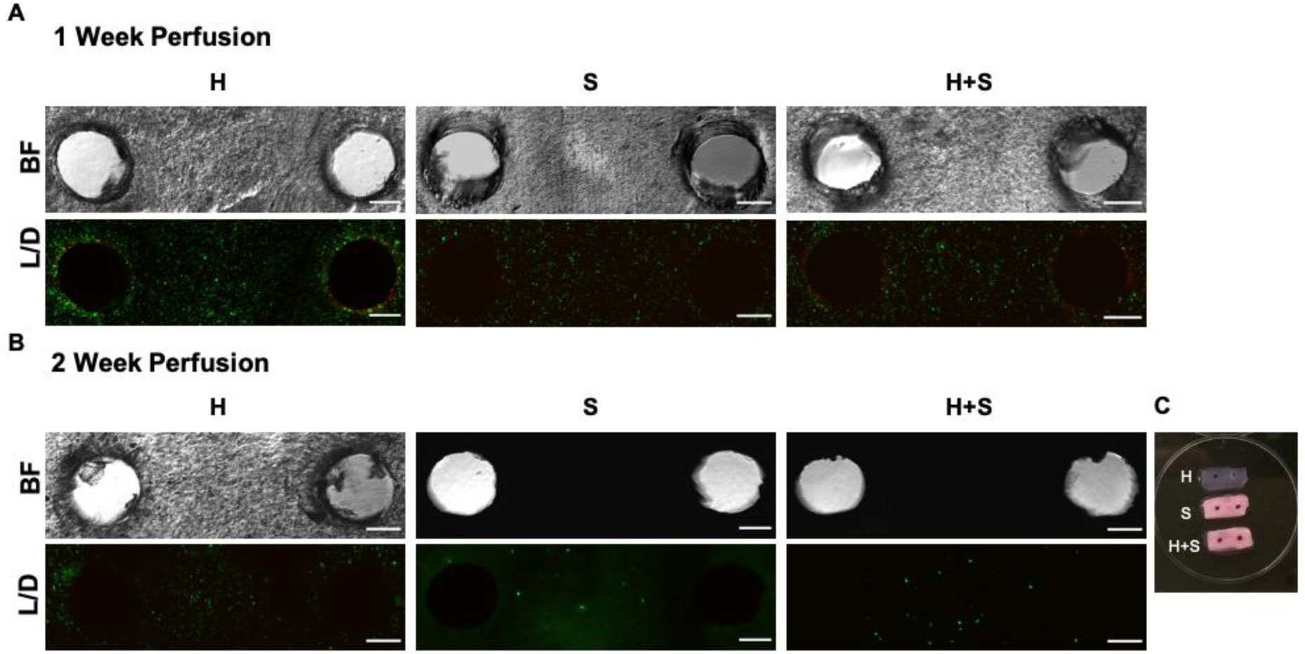
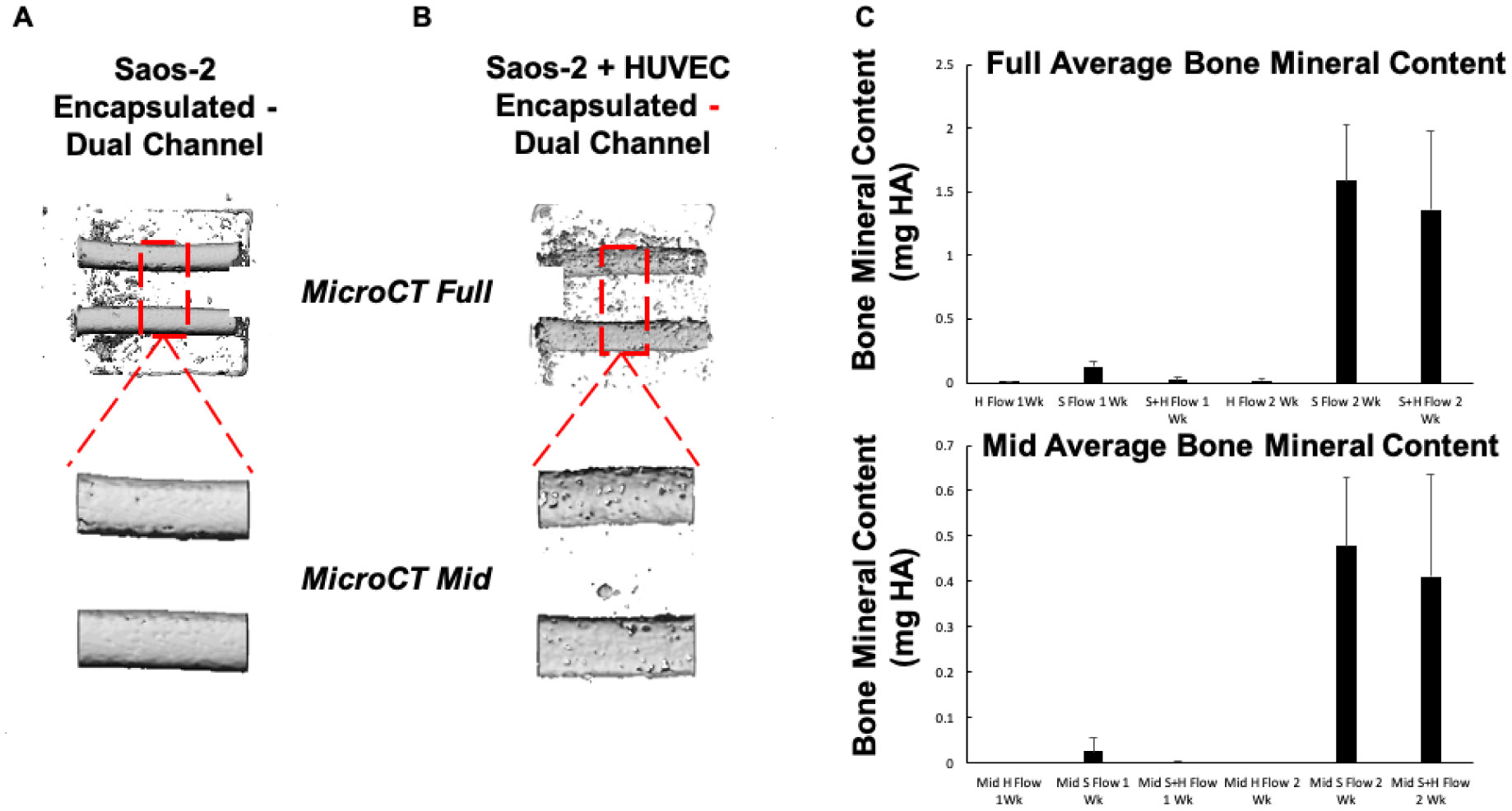
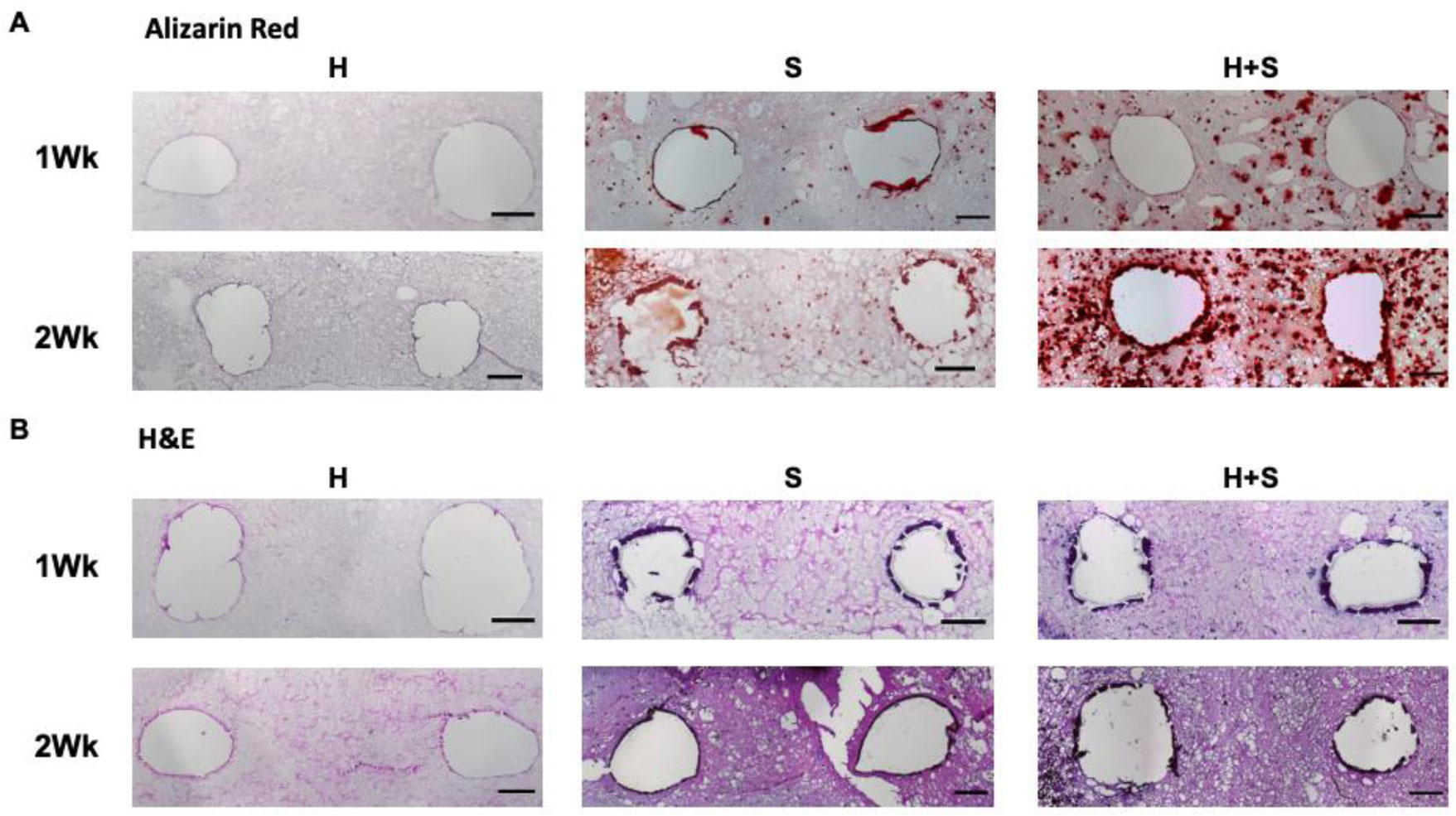
In this work, we report on a perfusion-based co-culture system that could be used for bone tissue engineering applications. The model system is created using a combination of Primary Human Umbilical Vein Endothelial Cells (HUVECs) and osteoblast-like Saos-2 cells encapsulated within a Gelatin Methacrylate (GelMA)-collagen hydrogel blend contained within 3D printed, perfusable constructs. The constructs contain dual channels, within a custom-built bioreactor, that were perfused with osteogenic media for up to two weeks in order to induce mineral deposition. Mineral deposition in constructs containing only HUVECs, only Saos-2 cells, or a combination thereof was quantified by microCT to determine if the combination of endothelial cells and bone-like cells increased mineral deposition. Histological and fluorescent staining was used to verify mineral deposition and cellular function both along and between the perfused channels. While there was not a quantifiable difference in the amount of mineral deposited in Saos-2 only versus Saos-2 plus HUVEC samples, the location of the deposited mineral differed dramatically between the groups and indicated that the addition of HUVECs within the GelMA matrix allowed Saos-2 cells, in diffusion limited regions of the construct, to deposit bone mineral. This work serves as a model on how to create perfusable bone tissue engineering constructs using a combination of 3D printing and cellular co-cultures.

Keywords:

Citation: Stephen W. Sawyer, Kairui Zhang, Jason A. Horton, Pranav Soman. Perfusion-based co-culture model system for bone tissue engineering[J]. AIMS Bioengineering, 2020, 7(2): 91-105. doi: 10.3934/bioeng.2020009

Related Papers:

[1]	Fisnik Morina, Simon Grima . The impact of pension fund assets on economic growth in transition countries, emerging economies, and developed countries. Quantitative Finance and Economics, 2022, 6(3): 459-504. doi: 10.3934/QFE.2022020
[2]	Oleg S. Sukharev . Economic crisis as a consequence COVID-19 virus attack: risk and damage assessment. Quantitative Finance and Economics, 2020, 4(2): 274-293. doi: 10.3934/QFE.2020013
[3]	Iuliana Matei . Is financial development good for economic growth? Empirical insights from emerging European countries. Quantitative Finance and Economics, 2020, 4(4): 653-678. doi: 10.3934/QFE.2020030
[4]	Naliniprava Tripathy . Does measure of financial development matter for economic growth in India?. Quantitative Finance and Economics, 2019, 3(3): 508-525. doi: 10.3934/QFE.2019.3.508
[5]	Ikram Ben Romdhane, Mohamed Amin Chakroun, Sami Mensi . Inflation Targeting, Economic Growth and Financial Stability: Evidence from Emerging Countries. Quantitative Finance and Economics, 2023, 7(4): 697-723. doi: 10.3934/QFE.2023033
[6]	Mustafa Hassan Mohammad Adam . Nexus among foreign direct investment, financial development, and sustainable economic growth: Empirical aspects from Sudan. Quantitative Finance and Economics, 2022, 6(4): 640-657. doi: 10.3934/QFE.2022028
[7]	Akash Deep . Advanced financial market forecasting: integrating Monte Carlo simulations with ensemble Machine Learning models. Quantitative Finance and Economics, 2024, 8(2): 286-314. doi: 10.3934/QFE.2024011
[8]	Sofía Orazi, Lisana B. Martinez, Hernán P. Vigier . Determinants and evolution of financial inclusion in Latin America: A demand side analysis. Quantitative Finance and Economics, 2023, 7(2): 187-206. doi: 10.3934/QFE.2023010
[9]	Md Qamruzzaman, Jianguo Wei . Do financial inclusion, stock market development attract foreign capital flows in developing economy: a panel data investigation. Quantitative Finance and Economics, 2019, 3(1): 88-108. doi: 10.3934/QFE.2019.1.88
[10]	Miquel Carreras-Simó, Germà Coenders . The relationship between asset and capital structure: a compositional approach with panel vector autoregressive models. Quantitative Finance and Economics, 2021, 5(4): 571-590. doi: 10.3934/QFE.2021025

Abstract

1. Introduction

Investments have a determining effect on economic dynamics. This influence unfolds in two main directions. Firstly, the dynamics of current investment spending contributes to the rate of economic growth. Secondly, investments in non-financial assets provide their expansion, which creates an opportunity for economic growth in the future. There are a lot of studies on the issue of assessing the impact of investments on economic development, in particular, public and private investments, which show different growth effects (Afonso and Aubyn, 2019; Chu, 2020), or emphasizing the negative impact of government spending on investments (Afonso and Jalles, 2015), for example, increasing social spending, which has an inhibitory effect on private investment and health care costs, according to the study, are recognized as having a positive effect on private investment. However, investments are not only public or private, but also in financial and non-financial assets.

Moreover, such a distribution of investments (structure) can significantly affect the economic dynamics. A significant increase in financial investments can be achieved by diverting the corresponding resources from investments in non-financial assets, which will affect the development of non-financial assets and the economic development opportunities. Of course, it is important how financial investments are adsorbed in the economy and how much they manage to subordinate to the tasks of developing the corporate sector. Consequently, changes in the financial and economic structure (Allen et al., 2018) determine one another in a certain way. The effect of determining changes in the economic structure (Zeira and Zoabi, 2015), applied to financial institutions and capital markets, is confirmed for a number of countries when considering a rather large sample of countries (Allen et al., 2018). However, the financial structure also affects economic growth (Chu, 2020), transforming especially strongly during the banking crisis, when the imbalance in the financial structure eliminates the positive effect of the influence of the securities market, or the influence of the banking sector on economic growth intensifies or decreases (Ghosh, 2017; Pradhan et al., 2017a, 2017b).

Thus, a large sample of countries showed that the banking sector has a negative impact on agriculture, especially where it is well developed, and does not have any negative or positive effect on industrial development (Tongurai and Vithessonthi, 2018). In turn, the authors substantiate the positive impact of industry on the development of the banking sector. Such approaches are useful for understanding not only the properties of economic dynamics, but also the emerging quality of the economy and structural ties. In countries with emerging markets, an unstable financial system and low banking sector potential, usually characterized by low incomes, banking sector growth hinders economic growth (Ghosh, 2017). Consequently, the effects of globalization of finance can adversely affect economic growth (Ghosh, 2017). In this vein, the urgent task is to assess the impact of financial and non-financial investments on economic dynamics. On the one hand, the principal characteristic for the country is the ratio of these investments. On the other hand, the sensitivity of GDP to these investments will be a measure of the degree of influence, taking into account the possible coherence between the dynamics of the two types of investments. The effect of private loan growth without increasing production volume negatively affects growth (Ductor and Grechyna, 2015). This is a demonstration of the impact of financial development on economic growth in terms of private lending and its proportionality to production growth. However, the impact of loans is measured in time, as well as their effect on the volume of production, although investments in non-financial assets also have both current and long-term effects on their impact on the economy. Moreover, it can be assumed that for investments in financial assets, the long-term effect is less pronounced.

Studies of the impact of the financial sector on economic dynamics can be represented in the form of three main groups.

Firstly, studies of the mutual influence of finance and growth, depending on whether the development of the financial sector is determined by the stock market or the banking system, or both (Peia and Roszbach, 2015; Bangake and Eggoh, 2011). The works (Mollaahmetoğlu and Akç alı, 2019; Botev et al., 2019; Hu et al., 2019) examine the relationship between financial development, financial innovation and economic growth. It has been determined that financial development and financial innovation have a significant impact on economic growth. An assessment of the impact of financial flows and their composition on the real exchange rate and economic growth is given in (Combes et al., 2019). The results show that net financial flows influence economic growth both directly and indirectly and the instability of market flows, such as FDI and portfolio investment, exacerbates the volatility of economic growth.

Improvement of economic growth indicators depending on financial development is shown in the study (Yıldırım et al., 2020). Here is an analysis of the impact of natural resource revenues on the financial development of developing countries that receive income from natural resources. Empirical results have shown that an increase in oil revenues has a positive impact on financial development in the long term. However, in the short term, rents for natural resources do not affect financial development. Income from natural resources is one of the main sources that can be used in the development of financial systems in these countries. However, from our point of view, this approach should have considered the impact on non-financial investments, which may depend as much as the financial system on the amount of income received from natural resources in such countries. In addition, the question of financial development and its success in the long term cannot be unrelated to the problem of general economic development and non-financial investments, which play a central role. In our study we do not consider factors that affect the financial system or non-financial investments, but rather the impact of financial and non-financial investments on economic dynamics.

The study (Kavya and Shijin, 2020) is considered the relationship between economic and financial development in relation to income inequality, taking into account the hypotheses of Kuznets, Greenwood. The results of the study indicate that there is no clear evidence that economic development and financial growth would reduce the problem of income inequality. Moreover, in most high-income developed countries financial development is not so great. This study highlights the need for further study on the impact of financial and non-financial investments on economic growth and not just in relation to the distribution of income or its value. In our opinion, such studies should include an assessment of the impact of financial and non-financial development opportunities on growth. Therefore, the study undertaken in this article becomes very useful from this point of view. Of course, there are articles that include the impact of certain subsystems, in particular, the banking system, on macroeconomic dynamics.

Thus, the study (Mensi and Hammoudeh, 2020) is considered the non-linear relationship between the development of the banking sector, the main macroeconomic indicators and economic growth in Islamic countries. The results show a positive non-linear relationship between the development of the banking sector and economic growth. In addition, the relationship between macroeconomic variable values and economic growth is asymmetric. Foreign direct investment, oil production and inflation have a positive impact on economic growth during a period of stable financial development, while state consumption and terms of trade have a negative impact on economic growth. The human capital index, education and the rule of law have little impact, regardless of the prevailing regime. Consequently, the stability of the financial system affects economic development in one way or another, which can be seen in various studies, but financial investments can act as a kind of indicator of such stability, which important to consider together with non-financial investments.

Secondly, the identification of imbalances between the financial and real sectors of the economy and their impact on economic growth (Ibrahim and Alagidede, 2018), for example, inhibition of innovation (Zhu et al., 2020). An assessment of financial innovation on economic growth is also presented in (Bernier and Plouffe, 2019), which shows the positive relationship between financial innovation and gross capital formation.

Thirdly, consideration of acceleration or inhibition of growth depending on changes in relevant parameters of the financial, banking system or stock market, insurance market or bond market, for example, lending volume, or the stability of the stock market or banking system (Beck et al., 2014) or previously unaccounted for factors becoming the most relevant (Nguyen et al., 2019).

These study groups suggest the use of various econometric methods (Bucci and Russo, 2019), but country samples are successfully analyzed using a panel vector autoregressive model to check Granger causality (Pradhan, et al., 2017b; Swamy and Dharani, 2019). In this study a statistically verified selection of the investment function describing the dynamics of GDP implemented in three countries—the USA (the country is the world leader), Germany (the economic leader of Europe) and Russia, is used as an econometric method of study. For these countries on the basis of obtaining the dynamics of GDP, which depends on investments in financial and non-financial assets, and also taking into account the displacement of the financial sector relative to the non-financial, a comparative description of the degree of influence on the economic dynamics of countries is given.

Summarizing what has been said, this allows to solve the problem of determining the correlative effect of investments in financial and non-financial assets on the economic dynamics of countries, which is the main goal of the study. According to the World Bank and the IMF guidelines, investments in financial assets are understood as instruments of participation in capital and units of investment funds, debt securities, options, forward contracts, other financial assets and liabilities¹. Investments in non-financial assets are understood as expenses on replenishment of fixed assets of the economy plus net changes in stock levels².

¹Source: World Bank https://data.worldbank.org/indicator/NE.GDI.TOTL.ZS, International Monetary Fund http://data.imf.org/regular.aspx?key=61545867.

² Source: Ibid. The study equally applies to the expressions financial and non-financial investments and investments in financial and non-financial assets respectively.

In contrast to the above studies, the authors in this article form, which is the originality of the proposed solution, a general algorithm for conducting study on the impact of financial and non-financial investments on the dynamics of GDP. This is done taking into account the changes in the introduced indicator of financial market bias, the obtained polynomial econometric models for the countries, and a model assessment of the contribution of two types of investments to their economic growth is given according to the structural formula. Thus, it is possible to assess the impact of each type of investment on economic dynamics, and to evaluate the accuracy of the models used. The proposed approach can be used for investment policy and for forecasts of changes in the growth rate when each type of investment changes.

The ratio of these investments can be a macroeconomic characteristic and be used when comparing the development of different countries. For example, the outstripping growth of financial investments relative to investments in non-financial assets indicates a shift in development focus towards the financial sector. This can both lead to inhibition of the overall dynamics, and in some cases contribute to it. In this regard, for further analysis, we formulate the main provisions of the applied methodology, which is reduced to the building of econometric models of the dynamics of the gross domestic product (GDP) depending on the two types of investments, as well as the use of a regression apparatus, which makes it possible to establish the sensitivity of these investments and the dynamics of GDP (growth rate) to change relevant parameters.

2. Research methodology and its algorithm

An econometric approach is applied to the study of the impact of investments in financial and non-financial assets on economic dynamics, which allows to link the change in the main macroeconomic indicator with these investments. Structural analysis is also useful, which allows to establish the ratio between the values of investments in financial assets and non-financial investments, which can be represented by the following indicator (formula (1)), which we denote as the displacement of the financial market (Sukharev, 2019):

$\gamma_{0} = \frac{F}{S-N}$

(1)

where:

F and N are the values of investments in financial and non-financial assets respectively;

S is the value of total savings.

It should be noted that in the general sense, the difference between the value of savings and non-financial investments is not equal to zero. Thus, savings are not equal to non-financial investments. If there is a point (year) where they are equal, then the analysis should be carried out by the inverse value of the indicator over the entire interval, adjusting the estimate taking into account this appeal. In this case the difference will be in the numerator and a decrease in the indicator and not its increase, will mean a shift in favor of the financial sector. In this study the equality of savings and non-financial investments was not observed in any of the years considered, therefore, the introduced indicator is used.

This indicator reflects the superiority of investments in financial assets over the difference between savings and non-financial investments. Differentiating the indicator of the financial market shift in time, accepting the condition when it grows, we obtain the following ratio:

${g}_{\gamma 0} \gt 0\\ {g}_{F} \gt \frac{{g}_{S}-n{g}_{N}}{1-n}$

(2)

where: ${g}_{F}, {g}_{N}$ are investment growth rates in financial and non-financial assets respectively;

$n = \frac{N}{S}$ , ${g}_{\gamma 0}$ is growth rate of financial market bias.

It follows from formula (2) that the growth rate of financial investments in order for the financial market shift to increase must exceed the difference between the weighted growth rates of savings and non-financial investments, where the weighting coefficient for the growth rate of savings is $\frac{1}{1-\mathrm{n}}$ , for the growth rate non-financial investments $\frac{\mathrm{n}}{1-\mathrm{n}}$ . If the displacement of the financial market is reduced, then the sign in inequality (2) is reversed.

Investments in non-financial assets N > S may exceed the amount of savings, then ${\mathrm{\gamma }}_{0} < 0$ . In this case the indicator will be negative. This in essence means that capital stays in the economy, exceeds the value of savings (it acts in the direction of revaluation of the national currency). If the negative value of the financial market shift indicator increases, then this indicates that with the superiority of non-financial investments over savings, which may increase, financial investments increase more significantly, or the superiority decreases (due to a corresponding change in non-financial investments or savings), while maintaining negative values of the indicator. At the same time financial investments may not grow, or even decrease by a certain amount.

In other cases, it has positive values, and it grows when the value of financial investments increases and when investments in non-financial assets increase, or savings decrease. It decreases if investments in financial assets and non-financial assets decrease (with the same amount of savings), or savings increase (with the same amount of non-financial investments). By this indicator, it can evaluate the shift—an increase or decrease in the influence of the financial market in the economy. An increase in the indicator indicates an increase in this influence, a decrease in the indicator indicates a decrease in this influence.

Changes in interest rates and the risk of financial and non-financial investments will have a significant impact on the dynamics of the indicator. Usually, at a lower interest rate on a loan, more investment is made. Also, with a higher dividend per share, investment in these securities becomes more attractive, which increases financial investments.

An econometric study of the impact of financial and non-financial investments on GDP involves the building of econometric models, their testing and verification.

The general algorithm of econometric study used in this article is reduced to the following steps:

(1) Formulation of the hypothesis about the relationship between changes in GDP, financial and non-financial investments.

(2) Model econometric building using the Ordinary Least Squares (OLS) for each country, but of an identical type, with their testing according to statistical criteria (shown below) that allow verification.

(3) Confirmation of verification of models and hypotheses of the study according to the set of statistical tests.

Then, models are applied to evaluate the contribution of investment to the rate of economic growth and obtain diagrams showing the impact of each type of investment on the growth rate.

To model building the OLS is used. This mathematical method is one of the basic methods of regression analysis. Using it, the authors determined the parameters of the model that best describes the development trend of the parameters. The goal of the OLS is precisely to find the best or optimal model. In this case the model will be optimal if the sum of the square deviations between the observed actual values and the corresponding calculated values is the minimum (smallest). OLS allowed to use the actual data to select an analytical function that runs as close to the actual points as possible.

These three positions of econometric study (building, testing and verification) constitute the stages of its implementation in the article. At the first stage, we assume that changes in GDP are related to two types of investment—financial and non-financial. The selection of models is carried out by the rejection method based on the best result determined using statistical tests. The regression analysis carried out to establish a close relationship between the relevant parameters to confirm the effectiveness involves testing and verification using the criteria. The use of these criteria allows to speak about the effectiveness of the conducted regression analysis and confirms the reliability of meaningful results based on it.

Econometric models are based on data from official statistical services: World bank, International Monetary Fund, Eurostat, Rosstat and so on. For the study, the initial time series were reduced to a constant price.

An important problem of multi-factor analysis is the selection of the most significant factors and model building that determines the values of the modeled indicator depending on the values of these factors. The study uses a method for solving this problem based on a complete search of all possible combinations of factors in order to build the best model with a fixed number of factors, which allows to select the optimal model from the set of best models (rejection method) based on known criteria of significance.

To ensure the reliability of the results of econometric modeling, the models were checked for compliance with the basic assumptions of regression analysis. A necessary condition for the reliability of the model and the effectiveness of the obtained coefficient estimates is the absence of multicollinearity of factors, heteroscedasticity and autocorrelation in the model residuals. To check the built models for multicollinearity the analysis of correlation matrices was used. Testing for heteroscedasticity and autocorrelation was performed using the White and Durbin-Watson tests as the most common and universal criteria.

The results of testing the basic assumptions of regression analysis allow to conclude that the models presented in the study can be used to adequately describe the economic dynamics in the analyzed countries.

Time series for GDP, financial and non-financial investments for the countries are used to build models and perform the necessary calculations for them (the normative choice of these countries is explained below). Descriptive statistics of relevant parameters for building models and calculating them are provided in Tables 2-4.

Table 1. Criteria of significance of econometric modeling results.

Name of the criterion	Mathematical notation and formula	Economic substance
Determination coefficient	${R}^{2}=\frac{{\sum (\widehat{y}-\stackrel{-}{y})}^{2}}{{\sum (y-\stackrel{-}{y})}^{2}}$	Shows the percentage of variation in the resultant attribute Y under the influence of the factor attribute X
Adjusted coefficient of determination	${R}_{adj}^{2}=\frac{\frac{{\sum (\widehat{y}-\stackrel{-}{y})}^{2}}{n-m-1}}{\frac{{\sum (y-\stackrel{-}{y})}^{2}}{n-1}}$	Allows to take into account the ratio of the number of observations and the number of estimated parameters of the model when evaluating the quality of the model
F-test	${\mathrm{F}}_{\mathrm{ф}\mathrm{а}\mathrm{к}\mathrm{т}.}=\frac{\frac{{\sum (\widehat{\mathrm{y}}-\stackrel{-}{\mathrm{y}})}^{2}}{\mathrm{m}}}{\frac{{\sum (\mathrm{y}-\stackrel{-}{\mathrm{y}})}^{2}}{\mathrm{n}-\mathrm{m}-1}}$ . If ${\mathrm{F}}_{\mathrm{ф}\mathrm{а}\mathrm{к}\mathrm{т}.}>{\mathrm{F}}_{\mathrm{т}\mathrm{а}\mathrm{б}\mathrm{л}.},$ the statistical significance of the model is recognized	Allows to evaluate the quality of the regression model as a whole
Student t-test	${t}_{a}=\frac{a}{{m}_{a}}, {t}_{b}=\frac{b}{{m}_{b}},$ where ${m}_{a}=\sqrt{\frac{\sum {(y-\widehat{y})}^{2}}{n-2}\frac{\sum {x}^{2}}{n\sum {(x-\stackrel{-}{x})}^{2}}},$ ${m}_{b}=\sqrt{\frac{\sum {(y-\widehat{y})}^{2}}{(n-2)*\sum {(x-\stackrel{-}{x})}^{2}}}.$ If ${\mathrm{t}}_{\mathrm{ф}\mathrm{а}\mathrm{к}\mathrm{т}.}>{\mathrm{t}}_{\mathrm{т}\mathrm{а}\mathrm{б}\mathrm{л}.},$ then the statistical significance of the model parameter is recognized.	Allows to evaluate the quality of regression model parameters
Durbin-Watson test	$DW=\frac{\sum {({e}_{i}-{e}_{i-1})}^{2}}{\sum {e}_{i}^{2}}$ . The critical values d₁ and d₂ are determined based on a table for the required significance level α, the number of observations n, and the number of explanatory variables m.	Allows to determine whether there is an autocorrelation of residuals
White test	Estimation of the regression of squares of residuals to all regressors, their squares and pairwise products. ${ᵡ}_{actual.}^{2}>{ᵡ}_{\alpha; m-1}^{2}$ , then the heteroscedasticity of random errors is recognized.	Allows to determine the presence of random error heteroscedasticity

| Show Table

DownLoad: CSV

Table 2. Descriptive statistics on indicators Russia, 2000–2018, in 2005 prices.

Financial investment, mln ＄US		Non-financial investment, mln ＄US	GDP, mln ＄US	GDP growth rate, %
Average	24, 092.1	3, 642.2	24, 595.4	3.8
Standard error	4, 611.5	187.0	994.0	1.0
Median	17, 067.4	3, 880.6	26, 190.9	4.5
Mode	-	-	-	1.8
Standard deviation	20, 101.1	814.9	4, 445.1	4.2
Sample variance	404, 055, 652.1	664, 114.7	19, 759, 033.5	17.5
Excess	0.6	−1.1	−0.8	2.1
Asymmetry	1.0	−0.3	−0.8	−1.1
Interval	71, 489.2	2, 583.3	13, 556.6	17.8
Minimum	2, 738.5	2, 356.1	16, 069.1	−7.8
Maximum	74, 227.6	4, 939.5	29, 625.6	10.0
Largest(1)	74, 227.6	4, 939.5	29, 625.6	10.0
Smallest(1)	2, 738.5	2, 356.1	16, 069.1	−7.8
Significance (95.0%)	9, 688.4	392.8	2, 080.4	2.0

| Show Table

DownLoad: CSV

Table 3. Descriptive statistics on indicators Germany, 2000–2018, in 2005 prices.

Financial investment, mln ＄US		Non-financial investment, mln ＄US	GDP, mln ＄US	GDP growth rate, %
Average	1, 174, 695.8	704, 235.3	3, 456, 157.4	1.4
Standard error	69, 787.6	12, 861.4	59, 498.0	0.5
Median	1, 096, 846.2	712, 059.1	3, 441, 355.9	1.7
Mode	-	-	3, 176, 872.8	-
Standard deviation	304, 197.0	56, 061.7	259, 345.9	2.2
Sample variance	92, 535, 807, 884.6	3, 142, 910, 703.3	67, 260, 308, 599.6	4.6
Excess	−2.0	0.1	−1.0	5.7
Asymmetry	0.0	0.3	0.4	−1.9
Interval	737, 466.6	221, 606.5	815, 318.8	9.7
Minimum	802, 159.5	607, 251.0	3, 123, 907.8	−5.6
Maximum	1, 539, 626.2	828, 857.6	3, 939, 226.6	4.1
Largest(1)	1, 539, 626.2	828, 857.6	3, 939, 226.6	4.1
Smallest(1)	802, 159.5	607, 251.0	3, 123, 907.8	−5.6
Significance (95.0%)	146, 618.3	27, 020.9	125, 000.7	1.0

| Show Table

DownLoad: CSV

Table 4. Descriptive statistics on indicators United States, 2000–2018, in 2005 prices.

Financial investment, mln ＄US		Non-financial investment, mln ＄US	GDP, mln ＄US	GDP growth rate, %
Average	1, 342, 096.8	3, 166, 979.9	15, 186, 837.9	2.1
Standard error	130, 466.7	89, 243.6	344, 869.6	0.3
Median	1, 412, 434.4	3, 180, 302.0	15, 008, 011.9	2.2
Mode	-	-	-	-
Standard deviation	553, 523.2	378, 628.7	1, 463, 157.7	1.5
Sample variance	306, 387, 983, 708.9	143, 359, 700, 052.6	2, 140, 830, 578, 775.4	2.2
Excess	−1.5	−0.8	−0.6	4.3
Asymmetry	0.1	0.2	0.1	−1.7
Interval	1, 542, 787.0	1, 333, 909.6	5, 098, 013.1	6.7
Minimum	710, 163.6	2, 543, 942.2	12, 746, 261.7	−2.5
Maximum	2, 252, 950.6	3, 877, 851.7	17, 844, 274.7	4.1
Largest(1)	2, 252, 950.6	3, 877, 851.7	17, 844, 274.7	4.1
Smallest(1)	710, 163.6	2, 543, 942.2	12, 746, 261.7	−2.5
Significance (95.0%)	275, 260.6	188, 287.6	727, 611.2	0.7

| Show Table

DownLoad: CSV

Tables 2-4 provide descriptive statistics of the indicators used in this study for the analyzed countries. Thus, an important indicator is sample variance, which reflects the measure of data dispersion around the arithmetic mean. Based on Tables 2-4, the sample variance takes a fairly high value relative to the analyzed indicators, which shows how far apart the values of random variables are. The largest value of the sample variance relative to the average value of financial investments in the United States, which indicates an unstable trend of this indicator. From this point of view, the most stable financial investments are registered in Russia. A similar trend is typical for non-financial investments and GDP. The opposite dynamics is observed in the indicator of the GDP growth rate. So, the smallest deviations are in the US, the largest in Russia. The mode value can only be determined for Russia and it takes a value of 1.8%, i.e. this value is more common in the analyzed data set. In Germany and the United States, there is no repetition of GDP growth rates.

The kurtosis coefficient characterizes the fineness or flatness of the distribution, which is due to the different nature of grouping the values of the variable around the average. Thus, the GDP values in all the countries have a flat-top distribution, since the coefficient takes negative values. In Other words, the distribution of GDP by year is characterized by “blurring”. The GDP growth rate, on the contrary, is characterized by a positive coefficient of excesses in all countries, therefore, the distribution of values is incomplete, or “compact” distribution of values. A possible reason for this is the high degree of attraction of variables to the central trend.

The symmetry of the distribution relative to the mode is determined using the asymmetry coefficient. The distribution may have a negative or positive asymmetry. Positive symmetry with a steeper left and a flatter right wing is typical for financial investments in Russia and the United States, which indicates a “gravitation” of trends towards lower values. In Germany, the asymmetry coefficient is 0, which indicates that the distribution of values is symmetrical. Positive symmetry is typical for non-financial investments in Germany and the United States, as well as for the GDP of these countries. The GDP growth rate is characterized by a negative coefficient for the analyzed countries. Russia also has a negative coefficient in terms of non-financial investment and GDP. A negative coefficient shows the “gravitation” of indicators towards higher values.

Since the study uses a comparative econometric analysis, it is performed by time series for each country. A model is built for each country (object). This allows to see and evaluate the impact of each type of investment on economic growth. The use of time series by country is sufficient, based on the purpose and purpose of the study and its content, which involves comparing models for each country separately. The conducted regression analysis is verified using a set of statistical tests, its effectiveness is justified by the applied statistical criteria, which are contained in table 1, where the rationale for their application is also given. This eliminates the problems that usually arise with time series analysis (for example, multi-collinearity), but also reduces the cost of preparing panel data, the use of which in this study is not a panacea and even in some sense makes it difficult to compare. This means that the scale of the method, if panel data is used, does not correspond to the goal and task that can be achieved using simpler procedures. Moreover, the study involves the use of not only econometric procedures, but also comparative structural analysis, which provides direct non-model estimates. Therefore, “econometric complexity” should be adequate to the problem statement and solution, and not an end in itself.

In addition to the econometric approach, the study involves structural analysis, therefore, the apparatus used and the assessment of the reliability of the results is not determined by statistical criteria applied to simple econometric models, but contains accurate calculation and analytical estimates, which are also an additional argument in justifying the reliability of the result.

It should be borne in mind that for individual countries (as will be shown below, for example, for Russia) the value of financial investments may exceed GDP. A structural approach, showing the ratio of investments, becomes important along with the econometric method to assess the impact on economic dynamics. The simplest models with which can evaluate the impact of investments in financial ( $F$ ) and non-financial assets ( $N$ ) can be represented in the following two types. The models are based on the fact that they show the impact of financial and non-financial investments on the GDP (Y), are representable in the form of a polynomial and in a multiplicative form (Sukharev, 2020b):

(1) $Y = c+a*F+b*N$ , where $a, b, c$ are model coefficients; $Y$ is GDP; $F, N$ are financial and non-financial investments respectively;

(2) $Y = A{F}^{\alpha }*{N}^{\beta }$ , where $A$ is absolute term of an model; $\alpha, \beta$ are exponents in the investment function for GDP ( $Y$ ), or replacement rates for the relevant investments by analogy with the Cobb-Douglas function.

Having differentiated the value of the product over time and carried out the simplest transformations, it is not difficult to arrive at an expression for the rate of economic growth. From the first model, we obtain the structural formula for the economic growth rate (g) of the form:

$g = a*if*{g}_{F}+b*in*{g}_{N}$

(3)

where:

$if, in$ are shares of investments in financial and non-financial assets in GDP (Y);

${g}_{F} = \frac{1}{F}\frac{dF}{dt}, {g}_{N} = \frac{1}{N}\frac{dN}{dt}$ are growth rate of investments in financial and non-financial assets respectively.

Based on the second model, after differentiating the product, we obtain the growth rate (g) in the form of the following structural formula:

$g = \alpha *{g}_{F}+\beta *{g}_{N}$

(4)

Both structural formulas (3)-(4) were obtained on the basis of introduced econometric models linking GDP with financial and non-financial investments.

In fact, they show the contribution of financial and non-financial investments to the growth rate. The use of these structural formulas, unlike other empirical applications of a similar approach (Sukharev, 2020b), or the portfolio method (Sukharev, 2019) is entirely determined by the accuracy of the built econometric models, since differentiation, if the models are inaccurate, can significantly affect the pace changes to the parameters included in the model. The final section of the study will show the accuracy of estimating GDP growth rate according to these models. Our study is conducted in three countries—the United States, Germany and Russia³, covering the period 2000-2019⁴^, on which a comparative analysis of the impact of financial and non-financial investments on economic dynamics is carried out according to the following algorithm.

³ Countries for consideration are taken on the basis of considerations of influence on the world economy (USA), the European system (Germany) and because of the authors’ residence is Russia. For China, there is no comparable information on financial investments in the considered time interval, therefore, the second world economy was not included in the analysis. However, if there is statistical information, the approach developed in the article can be similarly applied to the Chinese economy.

⁴ The interval for countries may vary slightly due to the availability of statistical data, as can be seen in the calculated charts.

Firstly, the dynamics of financial and non-financial investments reduced to 2005 prices is analyzed, and the parameter of the financial market shift for each country is calculated. This makes accurate analytical estimates based on the available data series.

Secondly, an assessment is made of the regression relationship between the dynamics of financial and non-financial investments, and the effect of the displacement of the financial market on GDP growth. Regression analysis involves the selection of the regression rejection method at the best statistical tests. Each country has its own regression based on the purpose of comparative analysis, so data series for each country are used, rather than panel data. The resulting regressions are checked using the criteria listed above. It’s needed to get regressions for each country, not for a combined sample of data.

Thirdly, econometric models for linking GDP with financial and non-financial investments are being built with a subsequent assessment of the impact of each type of investment on this rate (contribution to the growth rate according to the structural formula (2)). The building of models is carried out by the method of rejection according to the best statistical indicators of verification. The method of pair correlations of the contribution of financial and non-financial investments to economic dynamics is an additional way to justify the degree of their influence. In addition, this method acts as an additional verifier for estimates obtained from the built econometric models and from the resulting ones.

The final part of the study discusses the results obtained in a comparative analysis of countries, with the establishment of a specific picture of the impact of financial investments on economic growth. The likelihood of the results is estimated based on the adequacy of the applied regression apparatus and structural analysis, which allows us to obtain an analytically accurate estimate. In fact, it strengthens the adequacy of the results of regression analysis. Based on the crisis of 2020 caused by a virus attack on the global economy, according to the built models, a scenario forecast for 2020 is carried out with a 5% reduction in investments in financial and non-financial assets compared to the previous year. In addition, a forecast for 2021 is also given based on a 1% increase in financial investments and a 2% decrease in investments in non-financial assets.

Next, we implement the points of the study algorithm indicated above.

3. Dynamics of financial and non-financial investments: USA, Germany, Russia

Analysis of the dynamics of financial and non-financial investments is reflected in Figure 1 for the United States, Germany and Russia. As it can be seen, investments in non-financial assets prevail in the USA, unlike Germany. For Russia in the considered time interval there is a sharp increase in financial investments, many times exceeding investments in non-financial assets, moreover, exceeding GDP by 2 times (Figure 2, right).

Figure 1. Financial and non-financial investments in 2005 prices of the USA (left), Germany (center), Russia (right), 2000-2018⁵.

DownLoad: Full-Size Img PowerPoint

⁵ Source: World Bank https://data.worldbank.org/indicator/NE.GDI.TOTL.KD, International Monetary Fund https://data.imf.org/regular.aspx?key=61545853. Rosstat https://www.gks.ru/investment_nonfinancial, https://www.gks.ru/folder/14476, https://www.gks.ru/storage/mediabank/tab 1(2).htm.

Figure 2. Financial investments to GDP, 2000-2019 (left)⁶, the financial market bias of the USA, Germany, Russia, 2002-2018 (on right)⁷.

DownLoad: Full-Size Img PowerPoint

⁶ Source: World Bank https://data.worldbank.org/indicator/NE.GDI.TOTL.KD, International Monetary Fund https://data.imf.org/regular.aspx?key=61545853.

⁷Source: World Bank https://data.worldbank.org/indicator/NE.GDI.TOTL.KD, https://data.worldbank.org/indicator/NY.GNS.ICTR.ZS, https://data.worldbank.org/indicator/NY.GDP.MKTP.KD, International Monetary Fund http://data.imf.org/regular.aspx?key=61545865.

In the US and German economies investments in financial assets do not exceed GDP (Figure 2, left). The calculation of the financial market bias γ₀, presented in Figure 2, on the right, reflects a high financial market bias relative to the non-financial sector of the economy for Russia, especially after 2009, a significant decrease in this bias for Germany in the field of positive values and a negative value for the US economy. This suggests that the US economy attracted capital that exceeded savings and the increase in the negative bias until 2014 was associated with both increased financial and non-financial investments, and its further increase with a decrease in financial investments (Figure 2, right; Figure 1, left). The value of two types of investments in the United States significantly exceeded the size of German investments and significantly the same types of investments in the Russian economy. Non-financial investments in Germany were inferior in dynamics to financial investments (Figure 1, center), which ultimately affected the change in the magnitude of the displacement of the financial market (Figure 2, right).

Thus, each of the countries under consideration demonstrated its own characteristics of the development of the financial market and the scale of influence of financial investments.

Figure 3 shows the dynamics of financial and non-financial investments in the USA, Germany and Russia, showing a different degree of sensitivity of changes in some investments when others change over the considered time interval. So, in the American economy, judging by the connection obtained in Figure 3a, a 1.6-fold increase in non-financial investments is accompanied by a 3-fold increase in financial investments. For the German economy (Figure 3, b), a 1.34-fold increase in non-financial investments is accompanied by a 2-fold increase in financial investments. The Russian economy is characterized by a sharp shift towards the financial market, so a 2-fold increase in non-financial investments is accompanied by an almost 12-fold increase in financial investments (Figure 3, c). Consequently, the sensitivity of financial investments to non-financial ones is about 1.49 for Germany, 1.875 for the USA and the highest for Russia, about 6.0.

Figure 3. Regression model⁸ of financial and non-financial investments in the USA (a), Germany (b), Russia (c).

DownLoad: Full-Size Img PowerPoint

⁸ Based on: World Bank https://data.worldbank.org/indicator/NE.GDI.TOTL.KD, International Monetary Fund https://data.imf.org/regular.aspx?key=61545853, Rosstat https://www.gks.ru/investment_nonfinancial, https://www.gks.ru/folder/14476.

In this regard investments in non-financial assets in Russia are less sensitive to financial investments than in the USA and Germany. In turn, in Germany non-financial investments are more sensitive to financial investments than in the United States.

The significance of regression models (Table 5) is checked using the F-test. The calculated value shown in the Table 5 is greater than the table value for a given significance level α = 0.05, therefore, the models shown in Figure 3 are significant.

Table 5. Econometric characteristics of the models in Figure 3.

Characteristics	Model 1: United States	Model 2: Germany	Model 3: Russia
F-test	33.5	24.3	31.4
D-W_calculated	1.5 Є [1.53; 2.47]	1.6 Є [1.53; 2.47]	1.6 Є [1.4; 2.6]
White test	χ2 _calc. = 16.2; χ2 _crit. = 27.6	χ2 _calc. = 18.7; χ2 _crit. = 28.9	χ2 _calc. = 10.2; χ2 _crit. = 28.9.

| Show Table

DownLoad: CSV

To test the hypothesis of the presence of autocorrelation of residues, the authors used the Durbin-Watson test. According to the Durbin-Watson table at m = 1 the critical points for the significance level 0.05 and the number of observations 19 were determined, while the calculated value fell within the range [d₂; 4-d₂], therefore, there are reasons to believe that there is no autocorrelation. This is one of the confirmations of the high quality of the model (Jeffrey, 2012).

The universal test for determining the heteroscedasticity of random model errors is the White test (Baltagi and Badi, 2011). The ratio of calculated and critical values for each model allowed us to accept the null hypothesis of homoscedasticity of the model, i.e. one of the key assumptions of the OLS—the condition of constancy of variances of random deviations is fulfilled. These calculations show the significance and adequacy of the models built by the authors.

Conducting the regression analysis of the relationship between the GDP growth rate of each country and the financial sector bias parameter γ0 (Figure 4, Table 6), we find the following property. At this point in time the increase in the displacement of the financial market for the Russian economy (Figure 4, c) accompanied by a decrease in growth rate, the decline for the German an increase in the growth rate (Figure 4, b) and the American economy (Figure 4, a) some increase in growth rate. Comparing the change in the offset parameter with the dynamics of investments in financial and non-financial assets, it can get the final characteristic of the change in this parameter for a given economic dynamics. This characteristic is reflected in Table 7.

Figure 4. Regression model⁹ of the relationship between the economic growth rate and the displacement of the US financial market (a), Germany (b), Russia (c).

DownLoad: Full-Size Img PowerPoint

⁹ Based on: World Bank Всемирный банк https://data.worldbank.org/indicator/NE.GDI.TOTL.KD, https://data.worldbank.org/indicator/NY.GDP.MKTP.KD, International Monetary Fund https://data.imf.org/regular.aspx?key=61545853. Rosstat https://www.gks.ru/investment_nonfinancial, https://www.gks.ru/folder/14476, https://www.gks.ru/storage/mediabank/tab 1(2).htm.

Table 6. Econometric characteristics of the models in Figure 4.

Characteristics	Model 1: United States	Model 2: Germany	Model 3: Russia
F-test	8.4	11	11
D-W_calculated	1.4 Є [1.38; 2.62]	1.8 Є [1.38; 2.62]	1.8 Є [1.4; 2.6]
White test	χ2 _calc. = 17.4; χ2 _crit. = 27.6	χ2 _calc. = 9.9; χ2 _crit. = 26.3	χ2 _calc. = 11.3; χ2 _crit. = 28.9.

| Show Table

DownLoad: CSV

Table 7. Influence of financial market bias on economic dynamics (final assessment in Figure 4).

Country	Characteristics of the parameter γ0 influence on the economy dynamics
United States(2001–2018)	Non-financial investments predominate over financial investments and exceed savings, so that γ0 < 0 and grows due to the growth of financial investments. This is accompanied by a slight increase in the GDP growth rate.
Germany(2002–2018)	Financial investments prevail, but γ0 > 0 first decreases, then steadily due to non-financial investments. When it decreases, the growth rate increases.
Russia(2000–2018)	Very significant financial investments, exceeding non-financial ones, γ0 > 0 and increasing sharply due to the growth of financial investments. This shift in the financial market is accompanied by a slowdown in economic dynamics.

| Show Table

DownLoad: CSV

The predominance of financial investments is not a negative outcome for the economy, since the value of non-financial investments and the mutual influence of some on others is important. In particular, the German economy increased its pace with an average decrease in the size of the financial market bias. The US economy showed a negative value of the financial market shift, as capital flowed into the country and the total volume of non-financial investments exceeded savings. For the Russian economy, the sharp expansion of financial investment strongly affected the economic dynamics, which was accompanied by a decrease in the rate of economic growth (Figure 4, right).

Further, on the basis of econometric models built by the rejection method, we will show the contribution of each type of investment to the growth rate according to the obtained structural models (2). We will evaluate the accuracy of the models based on a combined estimate of the actual and estimated growth rate for each country. Let’s make a forecast for changes in GDP for the studied countries for 2020 and 2021, according to the scenario of a 5% decrease in investment of each type in the first year and a 2% decrease in non-financial investment with a 1% increase in financial investment in each country in 2021. We will calculate the decline in the rate and size of GDP in each country under this scenario, according to the built models. Let's summarize and discuss the results of the analysis.

4. Discussion

Let’s build econometric models of changes in the GDP of the United States, Germany and Russia depending on the size of financial and non-financial investments, focusing on the polynomial representation of the relationship (for the Russian economy, we will also include a multiplicative model of the relationship of these parameters). Next let’s estimate the contribution of investment to the growth rate of countries by dependencies (2) in Figure 6.

Figure 5. GDP dependence¹⁰ on investments in financial and non-financial assets of the United States (left), Germany (center), Russia (right) (Sukharev, 2020a).

DownLoad: Full-Size Img PowerPoint

¹⁰ Calculated by the authors from the source: World Bank https://data.worldbank.org/indicator/NE.GDI.TOTL.KD, https://data.worldbank.org/indicator/NY.GDP.MKTP.KD, International Monetary Funf https://data.imf.org/regular.aspx?key=61545853, Rosstat https://www.gks.ru/investment_nonfinancial, https://www.gks.ru/folder/14476, https://www.gks.ru/storage/mediabank/tab 1(2).htm.

Figure 6. The contribution of financial and non-financial investments to economic growth in the United States (left), Germany (center) and Russia (right)¹¹.

DownLoad: Full-Size Img PowerPoint

¹¹ Calculated by the authors from the source: World Bank https://data.worldbank.org/indicator/NE.GDI.TOTL.KD, https://data.worldbank.org/indicator/NY.GDP.MKTP.KD, International Monetary Fund https://data.imf.org/regular.aspx?key=61545853, Rosstat https://www.gks.ru/investment_nonfinancial, https://www.gks.ru/folder/14476, https://www.gks.ru/storage/mediabank/tab 1(2).htm.

Figure 5 shows the relationship between GDP and investment of two types. It can be seen, the accuracy of selecting models is very high.

The results of testing the main assumptions of regression analysis allow to conclude that for an adequate description of economic dynamics in the analyzed countries, the models presented in the study can be used, including for forecasting.

Comparing the dynamics of GDP in countries based on models that link the impact on GDP of financial and non-financial investments, we can conclude that with the same change in each type of investment in the United States, the impact on GDP change is quite close, and non-financial investments will have a stronger impact on its change. In Germany this influence will be even higher. However, in Russia, financial investment is most likely to affect the change in GDP in the direction of deceleration (Figure 5, right). It is noteworthy that if the US GDP declined in 2009, then in Russia both in 2009 and in 2015. (in Germany, we can also see a slowdown in GDP growth in 2005 prices in 2014-2015, Figure 5, center).

An important characteristic of the impact of financial and non-financial investments on economic dynamics is their contribution to the rate of economic growth. This contribution is calculated using structural formulas for each country and is shown in Figure 6 (using a polynomial model of the relationship between GDP and financial and non-financial investments). This is an analytically accurate calculation, the adequacy of which is checked by comparison with actual data and observed GDP dynamics. By itself, this approach provides information about the impact of each type of investment on the rate of economic growth, so that the regression apparatus, due to its inaccuracy in comparison with changes in real parameters, becomes a kind of auxiliary tool, but important, since analytically accurate estimates and models are combined. This can be seen by comparing the results. This creates an additional argument, in addition to statistical tests, to justify the adequacy of the use of regression models, which follows from the logic of comparative analysis.

As shown in Figure 6, according to the model used, the contribution of financial and non-financial investments varies over time in each country. Since 2014, the contribution to the growth rate, for example, in Russia is clearly more important than financial investment, in Germany, on the contrary, non-financial, in the United States-a very close contribution of both investments. The average contribution estimate for the period up to 2020 is shown in Table 2.

Figure 7 shows the calculation of the economic growth rate, compared with its actual values for countries. And for the United States and Germany, the rate calculated from the structural formula that meets the polynomial model (the most accurate), and for Russia—in the structural formula, corresponding multiplicative models of GDP from financial and non-financial investment (the accuracy of which is higher Figure 5, right).

Figure 7. Estimation¹² of the growth rate using the “structural formula” of the United States (left), Germany (center) and Russia (right) using the multiplicative model.

DownLoad: Full-Size Img PowerPoint

¹² Growth rate (y) is calculated based on the GDP model (Y).

As we can see, the use of the structural formula for estimating the GDP growth rate gives a very noticeable error, which is probably caused by the peculiarities of obtaining structural formulas (2)-(3) based on the differentiation of the built econometric model, which programs a certain degree of inaccuracy. Testing the structural formula on an empirical basis (Sukharev, 2020b) gives higher accuracy. However, for a number of points (Figure 7), the accuracy is quite high and in general, the quality parameters of the dynamics of the application of these formulas is quite reflected. It should be noted that the growth rate of the original model and the structural formula obtained from this model by differentiation are very precisely the same. Therefore, the inaccuracy of the initial econometric model creates a prerequisite for deviation from the actual data on the growth rate.

We will forecast the GDP growth rate for countries based on the scenario of a 5% reduction in financial and non-financial investments in 2020, due to a virus attack and a recession (a pessimistic scenario). In 2021 we will put an increase in financial investment by 1% and a reduction in non-financial investment by 2% due to the inertia of negative phenomena (we also take not the best option for restoring the world economy). The result is shown in Figures 8-10 for the United States, Germany and Russia. A polynomial model of changes in GDP from financial and non-financial investments was used to identify the comparison.

Figure 8. Forecast of the US GDP growth rate¹³.

DownLoad: Full-Size Img PowerPoint

¹³ Calculated by the authors from the source: World Bank https://data.worldbank.org/indicator/NE.GDI.TOTL.KD, https://data.worldbank.org/indicator/NY.GDP.MKTP.KD, International Monetary Fund https://data.imf.org/regular.aspx?key=61545853.

Figure 9. The forecast of GDP growth rate of Germany¹⁴.

DownLoad: Full-Size Img PowerPoint

¹⁴ Ibid.

Figure 10. Forecast of Russia’s GDP growth rate¹⁵.

DownLoad: Full-Size Img PowerPoint

¹⁵ Source: Rosstat https://www.gks.ru/investment_nonfinancial, https://www.gks.ru/folder/14476, https://www.gks.ru/storage/mediabank/tab 1(2).htm.

Let’s combine the data obtained for the forecast for 2020-2021 by country in the final Table 9, taking into account the contribution of financial investments to the economic dynamics of each country under consideration.

Table 8. Econometric characteristics of the models in Figure 5.

Characteristics	Model 1: United States	Model 2: Germany	Model 3: Russia
F-test	147	88.3	125.3
D-W_calculated	1.8 Є [1.53; 2.47]	1.9 Є [1.53; 2.47]	1.4 Є [1.4; 2.6]
White test	χ2 _calc. = 17.9; χ2 _crit. = 27.6	χ2 _calc. = 4.6; χ2 _crit. = 28.9	χ2 _calc. = 1.5; χ2 _crit. = 30.1

| Show Table

DownLoad: CSV

Table 9. Summary of scenario changes in the growth rate and the impact of financial and non-financial investments on the economic dynamics of countries.

Country	Scenario for 2020: reduction of financial and non-financial investments by 5% compared to the previous yearGrowth rate (the value of the previous year’s rate in 2019), %	Scenario for 2021: reduction of non-financial investments by 2%, growth of financial investments by 1% relative to 2020Growth rate, %	The average contribution of financial and non-financial investments to the growth rate in the considered interval for each country before the forecast, (forecast years 2020–2021), %
United States (2002-2019)	−3.09 (2.0)	−0.63	1.24; 1.02 (−0.38; −1.44)
Germany (2001–2019)	−3.22 (0.6)	−0.71	0.52; 0.46 (−0.37; −1.56)
Russia (2001–2019)	−3.54 (1.3)	−0.83	1.61; 2.04 (−0.37; -1.78)

| Show Table

DownLoad: CSV

As can be seen from Table 9, if financial and non-financial investment decreases by 5%, GDP will decline (the growth rate becomes negative) and the largest decline is observed where the financial sector has increased financial investment to the greatest extent relative to non-financial investment (as in Russia). While financial investment will grow by 1% next year, but non-financial investment will continue to decline by 2%, the model also shows a smaller decline in the countries considered, although the decline in Russia again remains the largest.

Figure 11 shows the change in the growth rate of the US economy (left), Germany (center) and Russia (right) according to the resulting econometric model for each country, based on the fact that the value of financial investments changes when non-financial investments are stable, or, conversely, non-financial investments change when the value of financial investments is stable. Thus, the obtained graphs allow to conclude about the impact on the growth rate of each type of investment, while the other type remains unchanged. In addition, they allow to compare this impact for the countries in question.

Figure 11. Change in the growth rate from changes in the type of investment in the United States (left), Germany (center), Russia (right)¹⁶.

DownLoad: Full-Size Img PowerPoint

¹⁶ Calculated by the authors from the source: World Bank https://data.worldbank.org/indicator/NE.GDI.TOTL.KD, https://data.worldbank.org/indicator/NY.GDP.MKTP.KD, International Monetary Funf https://data.imf.org/regular.aspx?key=61545853, Rosstat https://www.gks.ru/investment_nonfinancial, https://www.gks.ru/folder/14476, https://www.gks.ru/storage/mediabank/tab 1(2).htm.

Analyzing Figure 11, we conclude that a certain balance between financial and non-financial investments in the United States, with a decrease of some of their type by 5%, while other investments are stable, will lead to a smaller decrease in the growth rate, while maintaining it positive. In all the countries considered, it is the decline in non-financial investment that leads to a greater decrease in the rate than in financial investment and growth, accordingly, gives a greater rate. In Germany, a 5% decline in non-financial investment leads the rate to a negative value. In the Russian economy, due to the highest imbalance between financial and non-financial investments, even a small decline in financial and non-financial investments leads to negative growth rates according to the obtained model. The sensitivity of economies to non-financial investment also varies. So, with the growth of non-financial investments 5%, the lowest growth rate of discover the Russian economy, higher German and the highest rate—the US economy. The same applies to financial investments, although in Russia their value significantly exceeds the country’s GDP, in contrast to Germany and the United States. And the growth rate of the Russian economy will be much lower with the same increase in these investments in the countries considered.

Table 9, in its right column, gives an idea of the average contribution to the growth rate of the us, Germany and Russia. Despite the fact that non-financial investments predominate over financial investments in the US, their contribution [financial investments] to the growth rate is greater. For Russia, the situation is reversed: financial investments dominate in size over non-financial investments, but their average contribution to the growth rate in 2000-2019 is less than non-financial investments. For Germany, average deposits are quite close. For the forecast period 2020-2021. the main contribution to the decline in growth is made by non-financial investments and this negative contribution is crucial for the Russian economy. The impact of non-financial investments on the growth rate in a downturn is higher for all countries than for financial ones, although the contribution of financial investments in the US and Germany is higher on average for the period before the forecast, since the contribution also takes into account the growth rate of the investment itself. With each type of investment falling by 5%, the GDP decline is reflected in table 10.

Table 10. The amount of GDP decline with a 5% decrease in investment, us ＄ million in 2005 prices.

	Decrease in financial investments by 5% (non-financial-constant)	Reduction of non-financial investments by 5% (financial-constant)
Russia	−18, 406	−25, 860
Germany	−36, 703	−89, 667
United States	−179, 551	−385, 965

| Show Table

DownLoad: CSV

Table 10 shows that the largest absolute value of GDP decline is typical for the United States, the smallest-for Russia and with a reduction in non-financial investment, these losses in GDP are significantly higher for each country (but in relative change, as a share of GDP, they are higher for Russia). Although the absolute difference in losses for Russia when reducing each type of investment separately is the smallest of the three countries considered, the losses themselves are the highest as a share of GDP. The fact that this difference is the smallest is due to the characteristics of the resulting model relationship between GDP and the two types of investment.

Using the method of paired correlations, we obtain correlations of the contribution of financial and non-financial investments with the rate of economic growth for the United States, Germany and Russia for the period 2000-2019. The results are shown in Table 11-13.

Table 11. Paired correlations of investment contribution and growth rate, USA, 2002–2019.

	g	aifgF	bingN
g	1.00	0.33	0.73
aifgF	0.33	1.00	−0.38
bingN	0.73	−0.38	1.00

| Show Table

DownLoad: CSV

Table 12. Paired correlations of investment contribution and growth rate, Germany, 2001–2019.

	g	aifgF	bingN
g	1.00	0.52	0.93
aifgF	0.52	1.00	0.19
bingN	0.93	0.19	1.00

| Show Table

DownLoad: CSV

Table 13. Paired correlations of investment contribution and growth rate, Russia, 2001–2019.

	g	aifgF	bingN
g	1.00	0.23	0.95
aifgF	0.23	1.00	−0.08
bingN	0.95	−0.08	1.00

| Show Table

DownLoad: CSV

It follows from Table 11-13 that the contribution of non-financial investments has the greatest influence on the growth rate in Germany, and financial investments still have a significant impact on their contribution. In the US, the contribution of financial investment has less impact on the growth rate than in Germany and the same applies to non-financial investment. In the Russian economy, the contribution of non-financial investments has the greatest impact on the growth rate, and financial investments have the least impact in comparison with the United States and Germany. At the same time, the relationship between financial and non-financial investment contributions to the growth rate of the economy is very insignificant, even for the US, the pair correlation coefficient is -0.38.

This confirms the positions of the above analysis according to the applied econometric models.

Thus, the comparative econometric analysis of the impact of investments in financial and non-financial assets in the United States, Germany, and Russia allowed us to identify the significance and determine the degree of influence of the investment structure in terms of ensuring the economic growth of countries. The average growth rate in Russia was higher, but at the same time the financial economy was formed, with the development of which this growth slowed down. According to the obtained model, the largest decline in GDP is predicted for Russia in the event of a crisis. This is despite the fact that the contribution of non-financial investments to GDP dynamics is higher than financial ones. In Germany and the United States, the investment contribution is comparable, although the shift in the financial market relative to the non-financial market is less significant and did not increase significantly as in Russia. This circumstance can be considered as a determining condition for a strong downturn with the same decline in financial and non-financial investments in different countries. The sensitivity to this decline in GDP dynamics is different, since the structural structure is different. Consequently, one of the objectives of macroeconomic policies that stimulate growth and counteract decline is to correct the investment structure between financial and non-financial assets.

5. Conclusion

At the end of this study, we will summarize some of the most important results, which we will indicate in the form of three relevant positions.

First, financial investment, along with non-financial investment, can have a significant impact on economic dynamics, even if the economy is dominated by non-financial investment as a share of gross product. This influence is provided by the shift of the financial market relative to other economic sectors, that is, its advanced development, which does not always have a positive impact on the economy, as can be seen in the Russian economy.

Second, for the United States and Germany, the largest average contribution to the economic dynamics of financial investment is confirmed, regardless of the fact that the proportion between financial and non-financial investment for these countries is the opposite. In the US non-financial investments dominate, while in Germany, financial investments predominate. In Russia, financial investments are increasing sharply, but their impact on the growth rate is noticeable, but their contribution is 1.27 times less than the contribution of non-financial investments. This confirms the imbalance, reduced to unreasonable growth of the financial market (largest bias) in contrast to the United States and Germany, but this process is not related to the expansion of the influence on growth, unlike other countries surveyed, where the impact of the financial investment is large.

Third, the reduction of financial and non-financial investments in the context of the unfolding recession of 2020-2021 leads to a negative growth rate (according to the introduced scenario) for the three countries considered in 2020. An inertial reduction of non-financial investment by 2% in 2021, with an increase in financial investment by 1%, is also not able to bring these countries out of the expected recession. Consequently, an expansionary macroeconomic policy is required to stimulate non-financial and financial investments, and for the Russian economy, taking into account the sharp increase in the financial market bias, accompanied by measures to balance the financial sector relative to other sectors. Institutional measures that restrict the growth of the financial sector can change the built-up econometric relationship between gross product and types of investment, but in the long term they will increase the impact of non-financial investment on economic growth.

The prospects for further study work are actual problems of determining the most acceptable ratio between investments in financial and non-financial assets in terms of not only ensuring a certain amount of economic growth rate, but also the stability of this parameter, as well as ensuring the qualitative characteristics of economic development. In addition, one of the study areas may be to determine the sensitivity of each type of investment to macroeconomic policy measures. Moreover, it is important to take into account the balanced impact of each type of investment on the rate of economic growth. If there is a certain bias, for example, in the direction of financial investments, when their growth or decrease in the amount of savings, then this dynamics requires appropriate measures of macroeconomic policy to change the situation. The growth of non-financial investments is considered as a positive outcome for economic dynamics, however, if the bias parameter becomes negative, when these investments exceed the value of savings, the economy is dependent in its dynamics on external capital, which can also be considered as an unfavorable outcome that requires correction of economic policy.

Conflict of interest

All authors declare no conflicts of interest in this paper.

Acknowledgments

This work was supported by (IGERT) DMR-DGE-1068780. This work was also partially supported by NIH R21GM129607 awarded to Pranav Soman. We would like to thank the Syracuse University Machine Shop, Lucas D. Albrecht, and Alex B. Filip for creating the polycarbonate bioreactors and printing the ABS cages. We would also like to thank Professor Megan E. Oest from SUNY Upstate Medical University for their aid in microCT analysis and histological sectioning, and Professor Zhen Ma for the use of his fluorescence microscope.

Conflict of interest

The authors declare no conflict of interest.

Author contribution

S.W.S., K.Z. J.A.H and P.S. wrote the manuscript; S.W.S. J.A.H and P.S. conceived and designed the experiments; S.W.S. and K.Z. performed cell studies and analyzed results.

References

[1]	Buckwalter JA, Glimcher MJ, Cooper RR (1995) Bone biology. Part I: Structure, blood supply, cells, matrix, and mineralization. J Bone Joint Surg 77: 1256-1275. doi: 10.2106/00004623-199508000-00019
[2]	McCarthy I (2006) The physiology of bone blood flow: a review. JB & JS 88: 4-9.
[3]	Laroche M (2002) Intraosseous circulation from physiology to disease. Joint Bone Spine 69: 262-269. doi: 10.1016/S1297-319X(02)00391-3
[4]	Mercado-Pagán ÁE, Stahl AM, Shanjani Y, et al. (2015) Vascularization in bone tissue engineering constructs. Ann Biomed Eng 43: 718-729. doi: 10.1007/s10439-015-1253-3
[5]	Rouwkema J, Westerweel PE, De Boer J, et al. (2009) The use of endothelial progenitor cells for prevascularized bone tissue engineering. Tissue Eng Part A 15: 2015-2027. doi: 10.1089/ten.tea.2008.0318
[6]	Krishnan L, Willett NJ, Guldberg RE (2014) Vascularization strategies for bone regeneration. Ann Biomed Eng 42: 432-444. doi: 10.1007/s10439-014-0969-9
[7]	Shanjani Y, Kang Y, Zarnescu L, et al. (2017) Endothelial pattern formation in hybrid constructs of additive manufactured porous rigid scaffolds and cell-laden hydrogels for orthopedic applications. J Mech Behav Biomed Mater 65: 356-372. doi: 10.1016/j.jmbbm.2016.08.037
[8]	Murphy WL, Peters MC, Kohn DH, et al. (2000) Sustained release of vascular endothelial growth factor from mineralized poly (lactide-co-glycolide) scaffolds for tissue engineering. Biomaterials 21: 2521-2527. doi: 10.1016/S0142-9612(00)00120-4
[9]	Lee KY, Peters MC, Anderson KW, et al. (2000) Controlled growth factor release from synthetic extracellular matrices. Nature 408: 998-1000. doi: 10.1038/35050141
[10]	Sheridan MH, Shea LD, Peters MC, et al. (2000) Bioabsorbable polymer scaffolds for tissue engineering capable of sustained growth factor delivery. J Controll Release 64: 91-102. doi: 10.1016/S0168-3659(99)00138-8
[11]	Peters MC, Polverini PJ, Mooney DJ (2002) Engineering vascular networks in porous polymer matrices. J Biomed Mater Res A 60: 668-678. doi: 10.1002/jbm.10134
[12]	Wang L, Fan H, Zhang ZY, et al. (2010) Osteogenesis and angiogenesis of tissue-engineered bone constructed by prevascularized β-tricalcium phosphate scaffold and mesenchymal stem cells. Biomaterials 31: 9452-9461. doi: 10.1016/j.biomaterials.2010.08.036
[13]	Yu H, VandeVord PJ, Gong W, et al. (2008) Promotion of osteogenesis in tissue-engineered bone by pre-seeding endothelial progenitor cells-derived endothelial cells. J Orthop Res 26: 1147-1152. doi: 10.1002/jor.20609
[14]	Villars F, Bordenave L, Bareille R, et al. (2000) Effect of human endothelial cells on human bone marrow stromal cell phenotype: role of VEGF? J Cell Biochem 79: 672-685. doi: 10.1002/1097-4644(20001215)79:4<672::AID-JCB150>3.0.CO;2-2
[15]	Santos MI, Reis RL (2010) Vascularization in bone tissue engineering: physiology, current strategies, major hurdles and future challenges. Macromol Biosci 10: 12-27. doi: 10.1002/mabi.200900107
[16]	Villars F, Guillotin B, Amedee T, et al. (2002) Effect of HUVEC on human osteoprogenitor cell differentiation needs heterotypic gap junction communication. Am J Physiol-Cell Ph 282: C775-C85. doi: 10.1152/ajpcell.00310.2001
[17]	Stegen S, van Gastel N, Carmeliet G (2015) Bringing new life to damaged bone: the importance of angiogenesis in bone repair and regeneration. Bone 70: 19-27. doi: 10.1016/j.bone.2014.09.017
[18]	Ghanaati S, Fuchs S, Webber MJ, et al. (2011) Rapid vascularization of starch–poly (caprolactone) in vivo by outgrowth endothelial cells in co-culture with primary osteoblasts. J Tissue Eng Regen M 5: e136-e143. doi: 10.1002/term.373
[19]	Guillotin B, Bareille R, Bourget C, et al. (2008) Interaction between human umbilical vein endothelial cells and human osteoprogenitors triggers pleiotropic effect that may support osteoblastic function. Bone 42: 1080-1091. doi: 10.1016/j.bone.2008.01.025
[20]	Unger RE, Sartoris A, Peters K, et al. (2007) Tissue-like self-assembly in cocultures of endothelial cells and osteoblasts and the formation of microcapillary-like structures on three-dimensional porous biomaterials. Biomaterials 28: 3965-3976. doi: 10.1016/j.biomaterials.2007.05.032
[21]	Ma JL, van den Beucken JJJP, Yang F, et al. (2011) Coculture of osteoblasts and endothelial cells: optimization of culture medium and cell ratio. Tissue Eng Part C 17: 349-357.
[22]	Black AF, Berthod F, L'Heureux N, et al. (1998) In vitro reconstruction of a human capillary-like network in a tissue-engineered skin equivalent. FASEB J 12: 1331-1340. doi: 10.1096/fasebj.12.13.1331
[23]	Chiu LLY, Montgomery M, Liang Y, et al. (2012) Perfusable branching microvessel bed for vascularization of engineered tissues. Proc Natl Acad Sci USA 109: E3414-E3423. doi: 10.1073/pnas.1210580109
[24]	Zheng Y, Chen J, Craven M, et al. (2012) In vitro microvessels for the study of angiogenesis and thrombosis. Proc Natl Acad Sci USA 109: 9342-9347. doi: 10.1073/pnas.1201240109
[25]	Chen YC, Lin RZ, Qi H, et al. (2012) Functional human vascular network generated in photocrosslinkable gelatin methacrylate hydrogels. Adv Funct Mater 22: 2027-2039. doi: 10.1002/adfm.201101662
[26]	Cuchiara MP, Gould DJ, McHale MK, et al. (2012) Integration of self-assembled microvascular networks with microfabricated PEG-based hydrogels. Adv Funct Mater 22: 4511-4518. doi: 10.1002/adfm.201200976
[27]	Chrobak KM, Potter DR, Tien J (2006) Formation of perfused, functional microvascular tubes in vitro. Microvasc Res 71: 185-196. doi: 10.1016/j.mvr.2006.02.005
[28]	Price GM, Wong KHK, Truslow JG, et al. (2010) Effect of mechanical factors on the function of engineered human blood microvessels in microfluidic collagen gels. Biomaterials 31: 6182-6189. doi: 10.1016/j.biomaterials.2010.04.041
[29]	Nichol JW, Koshy ST, Bae H, et al. (2010) Cell-laden microengineered gelatin methacrylate hydrogels. Biomaterials 31: 5536-5544. doi: 10.1016/j.biomaterials.2010.03.064
[30]	Park JH, Chung BG, Lee WG, et al. (2010) Microporous cell-laden hydrogels for engineered tissue constructs. Biotechnol Bioeng 106: 138-148.
[31]	Sadr N, Zhu M, Osaki T, et al. (2011) SAM-based cell transfer to photopatterned hydrogels for microengineering vascular-like structures. Biomaterials 32: 7479-7490. doi: 10.1016/j.biomaterials.2011.06.034
[32]	Therriault D, White SR, Lewis JA (2003) Chaotic mixing in three-dimensional microvascular networks fabricated by direct-write assembly. Nat Mater 2: 265-271. doi: 10.1038/nmat863
[33]	Golden AP, Tien J (2007) Fabrication of microfluidic hydrogels using molded gelatin as a sacrificial element. Lab Chip 7: 720-725. doi: 10.1039/b618409j
[34]	Miller JS, Stevens KR, Yang MT, et al. (2012) Rapid casting of patterned vascular networks for perfusable engineered three-dimensional tissues. Nat Mater 11: 768-774. doi: 10.1038/nmat3357
[35]	Annabi N, Tamayol A, Uquillas JA, et al. (2014) 25th anniversary article: Rational design and applications of hydrogels in regenerative medicine. Adv Mater 26: 85-124. doi: 10.1002/adma.201303233
[36]	Bertassoni LE, Cardoso JC, Manoharan V, et al. (2014) Direct-write bioprinting of cell-laden methacrylated gelatin hydrogels. Biofabrication 6: 024105. doi: 10.1088/1758-5082/6/2/024105
[37]	Tan Y, Richards DJ, Trusk TC, et al. (2014) 3D printing facilitated scaffold-free tissue unit fabrication. Biofabrication 6: 024111. doi: 10.1088/1758-5082/6/2/024111
[38]	Wu W, DeConinck A, Lewis JA (2011) Omnidirectional printing of 3D microvascular networks. Adv Mater 23: H178-H183. doi: 10.1002/adma.201004625
[39]	Lee VK, Kim DY, Ngo H, et al. (2014) Creating perfused functional vascular channels using 3D bio-printing technology. Biomaterials 35: 8092-8102. doi: 10.1016/j.biomaterials.2014.05.083
[40]	Miller JS, Stevens KR, Yang MT, et al. (2012) Rapid casting of patterned vascular networks for perfusable engineered three-dimensional tissues. Nat Mater 11: 768-774. doi: 10.1038/nmat3357
[41]	Kolesky DB, Truby RL, Gladman AS, et al. (2014) 3D bioprinting of vascularized, heterogeneous cell-laden tissue constructs. Adv Mater 26: 3124-3130. doi: 10.1002/adma.201305506
[42]	Skardal A, Zhang J, McCoard L, et al. (2010) Photocrosslinkable hyaluronan-gelatin hydrogels for two-step bioprinting. Tissue Eng Part A 16: 2675-2685. doi: 10.1089/ten.tea.2009.0798
[43]	Gao Q, He Y, Fu J-z, et al. (2015) Coaxial nozzle-assisted 3D bioprinting with built-in microchannels for nutrients delivery. Biomaterials 61: 203-215. doi: 10.1016/j.biomaterials.2015.05.031
[44]	Yang L, Shridhar SV, Gerwitz M, et al. (2016) An in vitro vascular chip using 3D printing-enabled hydrogel casting. Biofabrication 8: 035015. doi: 10.1088/1758-5090/8/3/035015
[45]	Tocchio A, Tamplenizza M, Martello F, et al. (2015) Versatile fabrication of vascularizable scaffolds for large tissue engineering in bioreactor. Biomaterials 45: 124-131. doi: 10.1016/j.biomaterials.2014.12.031
[46]	Sawyer SW, Shridhar SV, Zhang K, et al. (2018) Perfusion directed 3D mineral formation within cell-laden hydrogels. Biofabrication 10: 035013. doi: 10.1088/1758-5090/aacb42
[47]	Sladkova M, De Peppo GM (2014) Bioreactor systems for human bone tissue engineering. Processes 2: 494-525. doi: 10.3390/pr2020494
[48]	Rice JJ, Martino MM, De Laporte L, et al. (2013) Engineering the regenerative microenvironment with biomaterials. Adv Healthc Mater 2: 57-71. doi: 10.1002/adhm.201200197
[49]	Cartmell SH, Porter BD, García AJ, et al. (2003) Effects of medium perfusion rate on cell-seeded three-dimensional bone constructs in vitro. Tissue Eng 9: 1197-1203. doi: 10.1089/10763270360728107
[50]	Albrecht LD, Sawyer SW, Soman P (2016) Developing 3D scaffolds in the field of tissue engineering to treat complex bone defects. 3D Print Addit Manuf 3: 106-112. doi: 10.1089/3dp.2016.0006
[51]	Hutmacher DW (2001) Scaffold design and fabrication technologies for engineering tissues—state of the art and future perspectives. J Biomater Sci Poly Ed 12: 107-124. doi: 10.1163/156856201744489
[52]	Burg KJL, Porter S, Kellam JF (2000) Biomaterial developments for bone tissue engineering. Biomaterials 21: 2347-2359. doi: 10.1016/S0142-9612(00)00102-2
[53]	Reichert JC, Hutmacher DW (2011) Bone tissue engineering. Tissue Engineering Heidelberg: Springer, 431-456. doi: 10.1007/978-3-642-02824-3_21
[54]	Bose S, Vahabzadeh S, Bandyopadhyay A (2013) Bone tissue engineering using 3D printing. Mater Today 16: 496-504. doi: 10.1016/j.mattod.2013.11.017
[55]	Stevens MM (2008) Biomaterials for bone tissue engineering. Mater Today 11: 18-25. doi: 10.1016/S1369-7021(08)70086-5
[56]	Baranski JD, Chaturvedi RR, Stevens KR, et al. (2013) Geometric control of vascular networks to enhance engineered tissue integration and function. Proc Natl Acad Sci USA 110: 7586-7591. doi: 10.1073/pnas.1217796110
[57]	Lee VK, Lanzi AM, Ngo H, et al. (2014) Generation of multi-scale vascular network system within 3D hydrogel using 3D bio-printing technology. Cell Mol Bioeng 7: 460-472. doi: 10.1007/s12195-014-0340-0
[58]	Sawyer S, Oest M, Margulies B, et al. (2016) Behavior of encapsulated saos-2 cells within gelatin methacrylate hydrogels. J Tissue Sci Eng 7: 1000173. doi: 10.4172/2157-7552.1000173
[59]	Sawyer SW, Dong P, Venn S, et al. (2017) Conductive gelatin methacrylate-poly (aniline) hydrogel for cell encapsulation. Biomed Phys Eng Express 4: 015005. doi: 10.1088/2057-1976/aa91f9
[60]	Mikos AG, Sarakinos G, Lyman MD, et al. (1993) Prevascularization of porous biodegradable polymers. Biotechnol Bioeng 42: 716-723. doi: 10.1002/bit.260420606

bioeng-07-02-009-s001.pdf

This article has been cited by:

1.	Lean Yu, Xiaowen Huang, Hang Yin, Can machine learning paradigm improve attribute noise problem in credit risk classification?, 2020, 70, 10590560, 440, 10.1016/j.iref.2020.08.016
2.	O. S. Sukharev, Investment Function of Economic Growth in Russia, 2021, 25, 2587-7089, 35, 10.26794/2587-5671-2021-25-1-35-50
3.	Feng Min, Fenghua Wen, Xiong Wang, Measuring the effects of monetary and fiscal policy shocks on domestic investment in China, 2022, 77, 10590560, 395, 10.1016/j.iref.2021.10.010
4.	Shuaishuai Jia, Hao Dong, Haowen Yang, Asymmetric Risk Spillover of the International Crude Oil Market in the Perspective of Crude Oil Dual Attributes, 2021, 9, 2296-665X, 10.3389/fenvs.2021.720278
5.	Qingqing Hu, Tinghui Li, Xue Li, Hao Dong, Dynamic Characteristics of Oil Attributes and Their Market Effects, 2021, 14, 1996-1073, 3927, 10.3390/en14133927
6.	Shuaishuai Jia, Hao Dong, Zhenzhen Wang, Identifying the Asymmetric Channel of Crude Oil Risk Pass-Through to Macro Economy: Based on Crude Oil Attributes, 2022, 9, 2296-598X, 10.3389/fenrg.2021.739653
7.	O. S. Sukharev, E. N. Voronchikhina, Financial Wealth in Macroeconomic Dynamics, 2022, 26, 2587-7089, 118, 10.26794/2587-5671-2022-26-2-118-135
8.	P.A IVANOV, INVESTMENT ACTIVITY OF TERRITORY: DEFINITION AND EVALUATION, 2021, 10, 23091762, 10.26140/anie-2021-1003-0037
9.	Peng Hou, Mengting Zhou, Jiaqi Xu, Yue Liu, Financialization, Government Subsidies, and Manufacturing R&D Investment: Evidence from Listed Companies in China, 2021, 13, 2071-1050, 12633, 10.3390/su132212633
10.	Li Xu, Ping Guo, Guoqin Pan, Effects of inter-industry agglomeration on environmental pollution: Evidence from China, 2023, 20, 1551-0018, 7113, 10.3934/mbe.2023307
11.	Tinghui Li, Xue Li, Khaldoon Albitar, Threshold effects of financialization on enterprise R & D innovation: a comparison research on heterogeneity, 2021, 5, 2573-0134, 496, 10.3934/QFE.2021022
12.	Yue Liu, Jinzhi Liu, Lichang Zhang, Enterprise financialization and R&D innovation: A case study of listed companies in China, 2023, 31, 2688-1594, 2447, 10.3934/era.2023124
13.	Min Hong, Jiajia He, Kexian Zhang, Zhidou Guo, Does digital transformation of enterprises help reduce the cost of equity capital, 2023, 20, 1551-0018, 6498, 10.3934/mbe.2023280
14.	Yanqiong Liu, Zhenghui Li, Yanyan Yao, Hao Dong, Asymmetry of Risk Evolution in Crude Oil Market: From the Perspective of Dual Attributes of Oil, 2021, 14, 1996-1073, 4063, 10.3390/en14134063
15.	Ali Hashemizadeh, Rana Umair Ashraf, Irfan Khan, Syed Anees Haider Zaidi, Digital financial inclusion, environmental quality, and economic development: the contributions of financial development and investments in OECD countries, 2023, 30, 1614-7499, 116336, 10.1007/s11356-023-30275-4
16.	Nazokat Amonova, ECONOMETRIC ANALYSIS OF THE IMPACT OF INVESTMENT FINANCING THROUGH MARKET MECHANISMS ON ECONOMIC DEVELOPMENT, 2023, 24, 2010-6130, 538, 10.55439/ECED/vol24_iss1/a84
17.	О. S. Sukharev, E. N. Voronchikhina, Inflation Targeting: Eliminating Economic Growth and Structural Deformation in Russia, 2024, 28, 2587-7089, 6, 10.26794/2587-5671-2024-28-1-6-19

Reader Comments

Your name:*

Email:*
© 2020 the Author(s), licensee AIMS Press. This is an open access article distributed under the terms of the Creative Commons Attribution License (http://creativecommons.org/licenses/by/4.0)