


Figure 1.
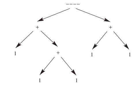
An expression tree for the number "$ [[1+[1+1]]----[1+1]] $".
Citation: Fatma Akpinar, Ayla Balci, Gulcan Ozomay, Ayca Sozen, Esra Kotan, Gulendam Kocak, Feyzullah Cetinkaya. Baby-skin care habits from different socio-economic groups and its impact on the development of atopic dermatitis[J]. AIMS Allergy and Immunology, 2018, 2(1): 1-9. doi: 10.3934/Allergy.2018.1.1
| [1] | Tareq M. Al-shami, Zanyar A. Ameen, A. A. Azzam, Mohammed E. El-Shafei . Soft separation axioms via soft topological operators. AIMS Mathematics, 2022, 7(8): 15107-15119. doi: 10.3934/math.2022828 |
| [2] | Mohammad H. M. Rashid, Feras Bani-Ahmad . An estimate for the numerical radius of the Hilbert space operators and a numerical radius inequality. AIMS Mathematics, 2023, 8(11): 26384-26405. doi: 10.3934/math.20231347 |
| [3] | Mustafa Ekici . On an axiomatization of the grey Banzhaf value. AIMS Mathematics, 2023, 8(12): 30405-30418. doi: 10.3934/math.20231552 |
| [4] | Thabet Abdeljawad, Kifayat Ullah, Junaid Ahmad, Muhammad Arshad, Zhenhua Ma . On the convergence of an iterative process for enriched Suzuki nonexpansive mappings in Banach spaces. AIMS Mathematics, 2022, 7(11): 20247-20258. doi: 10.3934/math.20221108 |
| [5] | Younes Talaei, Sanda Micula, Hasan Hosseinzadeh, Samad Noeiaghdam . A novel algorithm to solve nonlinear fractional quadratic integral equations. AIMS Mathematics, 2022, 7(7): 13237-13257. doi: 10.3934/math.2022730 |
| [6] | Jagdev Singh, Jitendra Kumar, Devendra kumar, Dumitru Baleanu . A reliable numerical algorithm based on an operational matrix method for treatment of a fractional order computer virus model. AIMS Mathematics, 2024, 9(2): 3195-3210. doi: 10.3934/math.2024155 |
| [7] | Amit K. Pandey, Manoj P. Tripathi, Harendra Singh, Pentyala S. Rao, Devendra Kumar, D. Baleanu . An efficient algorithm for the numerical evaluation of pseudo differential operator with error estimation. AIMS Mathematics, 2022, 7(10): 17829-17842. doi: 10.3934/math.2022982 |
| [8] | Mesfer H. Alqahtani, Alaa M. Abd El-latif . Separation axioms via novel operators in the frame of topological spaces and applications. AIMS Mathematics, 2024, 9(6): 14213-14227. doi: 10.3934/math.2024690 |
| [9] | Yonghong Duan, Ruiping Wen . An alternating direction power-method for computing the largest singular value and singular vectors of a matrix. AIMS Mathematics, 2023, 8(1): 1127-1138. doi: 10.3934/math.2023056 |
| [10] | Najla Altwaijry, Cristian Conde, Silvestru Sever Dragomir, Kais Feki . Further norm and numerical radii inequalities for operators involving a positive operator. AIMS Mathematics, 2025, 10(2): 2684-2696. doi: 10.3934/math.2025126 |
In [1], we distinguished the limit from the infinite sequence. In [2], we defined the Operator axioms to extend the traditional real number system. In [3], we promoted the research in the following areas:
1. We improved on the Operator axioms.
2. We defined the VE function and EV function. For clarity, we rename VE Function [3] to Prefix Function. For clarity, we rename EV Function [3] to Suffix Function.
3. We proved two theorems about the Prefix function and Suffix function.
The Operator axioms forms a new arithmetic axiom. The [3,Definition 2.2] defines real number system on the basis of the logical calculus $ \{ \Phi, \Psi \} $. The [2,TABLE 2] defines new operators according to the definition of number systems. Real operators naturally produce new equations such as $ y = [x++++[1+1]] $, $ y = [[1+1]----x] $, $ y = [x////[1+1]] $ and so on. In other words, real operators extend the traditional mathematical models which are selected to describe various scientific rules. Operator axioms have included infinite operators, so no other operator can be added to them. This means the Operator axioms is a complete real number system. In fact, infinite operators imply the completeness.
Thus, real operators exhibit potential value as follows:
1. Real operators can give new equations and inequalities so as to precisely describe the relation of mathematical objects.
2. Real operators can give new equations and inequalities so as to precisely describe the relation of scientific objects.
So real operators help to describe complex scientific rules which are difficult described by traditional equations and have an enormous application potential.
As to the equations including real operators, engineering computation often need the approximate solutions reflecting an intuitive order relation and equivalence relation. Although the order relation and equivalence relation of real numbers are consistent, they are not as intuitive as those of base-b expansions. In practice, it is quicker to determine the order relation and equivalence relation of base-b expansions. So we introduce numerical computations to approximate real numbers with base-b expansions.
The numerical computations we proposed are not the best methods to approximate real numbers with base-b expansions, but the simple methods to approximate real numbers with base-b expansions. The compution complexity of the numerical computations we proposed could be promoted furtherly. However, we first prove that the Operator axioms can run on any modern computer. The numerical computation we proposed blends mathematics and computer science. Modern science depends on both the mathematics and the computer science. Arithmetic is the core of both the mathematics and the science. As a senior arithmetic, the Operator axioms will promote both the mathematics and the science in the future.
Theorem 1.1. Any positive number $ \xi $ may be expressed as a limit of an infinite base-b expansion sequence
|
$ limn→∞A1A2⋯As+1. a1a2a3⋯an, $
|
(1.1) |
where $ 0 \leq A_{1} < b, 0 \leq A_{2} < b, \cdots, 0 \leq a_{n} < b $, not all A and a are 0, and an infinity of the $ a_n $ are less than (b-1). If $ \xi \geq 1 $, then $ A_{1} \geq 0 $.
Proof. Let $ [\xi] $ be the integral part of $ \xi $. Then we write
|
$ ξ=[ξ]+x=X+x, $
|
(1.2) |
where $ X $ is an integer and $ 0 \leq x < 1 $, and consider $ X $ and $ x $ separately.
If $ X > 0 $ and $ b^{s} \leq x < b^{s+1} $, and $ A_1 $ and $ X_1 $ are the quotient and remainder when $ X $ is divided by $ b^{s} $, then $ X = A_1 \cdot b^{s} + X_1 $, where $ 0 < A_1 = [b^{-s}X] < b $, $ 0 \leq X_1 < b^s $.
Similarly
|
$ X1=A2⋅bs−1+X2(0≤A2<b,0≤X2<bs−1),X2=A3⋅bs−2+X3(0≤A3<b,0≤X3<bs−2),⋯⋯⋯Xs−1=As⋅b+Xs(0≤As<b,0≤Xs<b),Xs=As+1(0≤As+1<b). $
|
Thus $ X $ may be expressed uniquely in the form
|
$ X=A1⋅bs+A2⋅bs−1+⋯+As⋅b+As+1, $
|
(1.3) |
where every $ A $ is one of 0, 1, $ \cdots $, (b-1), and $ A_1 $ is not 0. We abbreviate this expression to
|
$ X=A1A2⋯AsAs+1, $
|
(1.4) |
the ordinary representation of $ X $ in base-b expansion notation.
Passing to $ x $, we write
|
$ X=f1(0≤f1<1). $
|
We suppose that $ a_1 = [b f_1] $, so that
|
$ a1b≤f1<a1+1b; $
|
$ a_1 $ is one of 0, 1, $ \cdots $, (b-1), and
|
$ a1=[bf1],bf1=a1+f2(0≤f2<1). $
|
Similarly, we define $ a_2, a_3, \cdots $ by
|
$ a2=[bf2],bf2=a2+f3(0≤f3<1),a3=[bf3],bf3=a3+f4(0≤f4<1),⋯⋯⋯ $
|
Every $ a_n $ is one of 0, 1, $ \cdots $, (b-1). Thus
|
$ x=xn+gn+1, $
|
(1.5) |
where
|
$ xn=a1b+a2b2+⋯+anbn, $
|
(1.6) |
|
$ 0≤gn+1=fn+1bn<1bn. $
|
(1.7) |
We thus define a base-b expansion $.a_1 a_2 a_3 \cdots a_n \cdots $ associated with $ x $. We call $ a_1, a_2, \cdots $ the first, second, $ \cdots $ digits of the base-b expansion.
Since $ a_n < b $, the series
|
$ ∞∑1anbn $
|
(1.8) |
is convergent; and since $ g_{n+1} \rightarrow 0 $, its sum is $ x $. We may therefore write
|
$ x=. a1a2a3⋯, $
|
(1.9) |
the right-hand side being an abbreviation for the series (1.8).
We now combine (1.2), (1.4), and (1.9) in the form
|
$ ξ=X+x=A1A2⋯AsAs+1. a1a2a3⋯; $
|
(1.10) |
and the claim follows.
Theorem 1.1 implies that every real number has base-b expansions arbitrary close to it. So in numerical computations for the Operator axioms, all operands and outputs are denoted by base-b expansions to intuitively show the order relation and equivalence relation.
The paper is organized as follows. In Section 2, we define the operation order for all operations in the Operator axioms. In Section 3, we construct the numerical computations for binary operations. In Section 4, we define some concepts in the Operator axioms.
In the Operator axioms, the number '1' is the only base-b expansion while the others derive from the operation of two numbers and one operator. For example, the number "$ [[1+[1+1]]----[1+1]] $" derives from the operation of the number "$ [1+[1+1]] $", the number "$ [1+1] $" and the real operator "$ ---- $".
Definition 2.1. Numerical computation is a conversion from an operation to an approximate base-b expansion.
In general, an operation includes many binary operators. For example, the operation "$ [[1+[1+1]]----[1+1]] $" includes three "$ + $" and one "$ ---- $". Since each operator produces a binary operation, $ n $ operator in an operation will produce $ n $ binary operations. It is better to compute all binary operations in an operation in order. The order is denoted as Operation Order.
[4,§5.3.1] stores tradition operations as an expression tree and then applies traversal algorithm to evaluate the expression tree. Likewise, each operation of the Operator axioms can be stored as an expression tree in which each number '1' become a leaf node and each operator become an internal node. Then Operation Order is just the traversal order of the expression tree. In this paper, we choose inorder traversal as Operation Order. Figure 1 illustrates an expression tree for the number "$ [[1+[1+1]]----[1+1]] $".
It is supposed that the numerical computation applies base-10 expansions. Then the numerical computation for "$ [[1+[1+1]]----[1+1]] $" will proceed with the following Operation Order:
|
$ [[1+[1+1]]−−[1+1]]=[[1+2]−−−−[1+1]]=[3−−−−[1+1]]=[3−−−−2] $
|
In summary, every operation in the Operator axioms can divide into many binary operations by Operation Order. So numerical computations focus on the binary operations.
In [3], Operator axioms have expressed the real number system. In this section, "real number" refer to the real number deduced from Operator axioms [3].
According to the complexity of numerical computations, we divide binary operations into low operations, middle operations and high operations. Table 1 lists their elements in detail.
| Low operations | Middle operations | High operations | |
| Operators | $ +, ++, -, --, /, // $ | $ +++, ---, /// $ | $ ++++, +++++, \cdots, $ |
| $ ----, -----, \cdots, $ | |||
| $ ////, /////, \cdots $ |
 DownLoad:
CSV
DownLoad:
CSV
In the Operator axioms, $ / $ is equal to $ - $ while $ // $ is equal to $ -- $. From a traditional viewpoint, the low operations "$ +, ++, -, - $" are equal to basic arithmetic operations "$ +, \times, -, \div $". So numerical computations for low operations have been constructed in elementary arithmetic.
From a traditional viewpoint, $ +++ $ is an exponentiation operation, $ --- $ is a root-extraction operation and $ /// $ is a logarithm operation. In this subsection, we import the numerical computations for the middle operations "$ +++, ---, /// $" in [5,§23].
Let $ e $ be Euler's number. It is supposed that $ a \in \bigl(-\infty, +\infty\bigl) $ is a base-b expansion, $ n \in Z $ and $ k \in N $. The numerical computation for $ [e+++a] $ can be constructed with the Taylor-series expansion as follows.
|
$ [e+++a]=[limk→+∞(k∑n=0[[a+++n]−−[n!]])]≈[1+[a−−[1!]]+[[a+++2]−−[2!]]+[[a+++3]−−[3!]]+⋯+[[a+++n]−−[n!]]+⋯] $
|
It is supposed that $ a \in \bigl(0, +\infty\bigl) $ is a base-b expansion and $ n \in Z $. Let $ b = [[a-1]--[a+1]] $, then the numerical computation for $ [a///e] $ can be constructed with the Taylor-series expansion as follows.
|
$ [a///e]=[[[1+b]−−[1−b]]///e]=[2++[limk→+∞(k∑n=0[[b+++[2n+1]]−−[2n+1]])]]≈[2++[b+[[b+++3]−−3]+[[b+++5]−−5]+⋯+[[b+++[2n+1]]−−[2n+1]]+⋯]] $
|
It is supposed that $ a $ and $ b $ are two base-b expansions, where $ a \in \bigl(0, +\infty\bigl) $ and $ b \in \bigl(-\infty, +\infty\bigl) $. Then the numerical computation for $ [a+++b] $ can be divided and conquered with the identity $ [a+++b] = [e+++[b++[a///e]]] $.
It is supposed that $ [a+++b] $ is a real number, where $ a \in \bigl(-\infty, 0\bigl] $ and $ b \in \bigl(-\infty, +\infty\bigl) $ are two base-b expansions. Then the numerical computation for $ [a+++b] $ can always be equated with the basic numerical computations as above and the basic arithmetic operations in the axioms (OA.1)$ \sim $(OA.75).
It is supposed that the constants $ n, a_1, a_2, b_1, b_2, c_1, c_2, m \in N $.
Zero can be equated with a fraction $ [[1-1]--1] $. Any non-zero base-b expansion can be equated with a fraction $ [[1-1]\pm[a_1--a_2]] $ for $ a_1, a_2 \in N $.
It is supposed that the constant $ d \in R $ with $ [1-1] < d $. It is supposed that the constant $ e \in R $ with $ 1 < e $. For clarity, we rename VE Function [3] to Prefix Function. For clarity, we rename EV Function [3] to Suffix Function.
Definition 3.1. [3,Definition 3.1] Prefix Function is the function $ f : \bigl[1, +\infty\bigl) \rightarrow R $ defined by $ f(x) = [x+++\dot{e}d] $.
Definition 3.2. [3,Definition 3.2] Suffix Function is the function $ f : R \rightarrow R $ defined by $ f(x) = [e+++\dot{e}x] $.
Definition 3.3. [3,Definition 3.3] Fundamental operator functions are Prefix Function and Suffix Function.
Theorem 3.4. [3,Theorem 3.4] The Prefix Function $ f(x) = [x+++\dot{e}d] $ is continuous, unbounded and strictly increasing.
Theorem 3.5. [3,Theorem 3.5] The Suffix Function $ f(x) = [e+++\dot{e}x] $ is continuous, unbounded and strictly increasing.
It is supposed that the constant $ t, u, v \in R $.
Definition 3.6. Root Equations are the equations such as $ f(x) = t $ such that:
1. The function $ f(x) $ is real and continuous on any closed interval $ \bigl[u, v\bigl] $ in the domain;
2. The equation $ f(x) = t $ has only one root on the above interval $ \bigl[u, v\bigl] $;
[6,TABLE PT2.3] lists common root-finding methods and their convergence conditions. When $ a $ acts as the lower guess and $ b $ acts as the upper guess, both the bisection method [6,§5.2] and Brent's method [6,§6.4] always converge and find the only root on $ \bigl[u, v\bigl] $. But Brent's method converges faster than the bisection method and thus acts as the main root-finding method for Root Equations.
In the following, we construct all numerical computations for high operations by induction. It is supposed that the constant $ p_1 \in R $ with $ 1 \leq p_1 $. It is supposed that the constant $ p_2 \in R $. It is supposed that the constant $ q_1 \in R $ with $ 1 \leq q_1 $. It is supposed that the constant $ q_2 \in R $ with $ [1-1] \leq q_2 $. It is supposed that the constant $ r_1 \in R $ with $ [1-1] < r_1 $. It is supposed that the constant $ r_2 \in R $ with $ 1 < r_2 $. In the following, we approximate these constants with those fractions such as $ [a_1--a_2] $.
1. The numerical computations for the operations $ [p_1++++p_2] $, $ [q_1----q_2] $, $ [r_1////r_2] $ are constructed.
(a) A numerical computation for $ [[a_1--a_2]++++[b_1--b_2]] $ with $ 1 \leq [a_1--a_2] $ and $ [1-1] \leq [b_1--b_2] $ can be constructed.
i. $ [b_1--b_2] \leq 1 $.
|
$ (A1)(ˉc=[[[a1−−a2]−1]++[1+[1+1]]])∧(ˉd=[[[a1−−a2]−1]++[1+1]])∧(ˉe=[[b1−−b2]+++[1+1]])∧(ˉf=[[b1−−b2]+++[1+[1+1]]])∧([[a1−−a2]++++[b1−−b2]]=[[1+[ˉc++[ˉe+++1]]]−[ˉd++[ˉf+++1]]])by (OA.83), (OA.28)(A2)(ˉc=[[[a1−−a2]−1]++[1+[1+1]]])∧(ˉd=[[[a1−−a2]−1]++[1+1]])∧(ˉe=[[b1−−b2]+++[1+1]])∧(ˉf=[[b1−−b2]+++[1+[1+1]]])∧([[a1−−a2]++++[b1−−b2]]=[[1+[ˉc++ˉe]]−[ˉd++ˉf]])by (OA.83), (OA.62) $
|
ii. $ 1 < [b_1--b_2] $.
|
$ (B1)[[a1−−a2]++++[b1−−b2]]=[[a1−−a2]+++[[a1−−a2]++++[[b1−−b2]−1]]]by (OA.82)(B2)It is supposed that [1−1]≤[[b1−−b2]−n] and [[b1−−b2]−n]≤1. Let us distinguish these [a1−−a2] with the subscripts {(1),(2),(3),⋯}.(B3)⇒[[a1−−a2]++++[b1−−b2]]=[[a1−−a2](1)+++[[a1−−a2](2)+++⋯[[a1−−a2]n+++[[a1−−a2]++++[[b1−−b2]−n]]⋯]]by (OA.82), (B2)(B4)(ˉc=[[[a1−−a2]−1]++[1+[1+1]]])∧(ˉd=[[[a1−−a2]−1]++[1+1]])∧(ˉe=[[[b1−−b2]−n]+++[1+1]])∧(ˉf=[[[b1−−b2]−n]+++[1+[1+1]]])∧([[a1−−a2]++++[[b1−−b2]−n]]=[[1+[ˉc++ˉe]]−[ˉd++ˉf]])by (B2), (A2)(B5)⇒(ˉc=[[[a1−−a2]−1]++[1+[1+1]]])∧(ˉd=[[[a1−−a2]−1]++[1+1]])∧(ˉe=[[[b1−−b2]−n]+++[1+1]])∧(ˉf=[[[b1−−b2]−n]+++[1+[1+1]]])∧([[a1−−a2]++++[b1−−b2]]=[[a1−−a2](1)+++[[a1−−a2](2)+++⋯[[a1−−a2]n+++[[1+[ˉc++ˉe]]−[ˉd++ˉf]]⋯]])by (B3), (B4) $
|
Then (A1)$ \sim $(A2) and (B1)$ \sim $(B4) have reduced one $ ++++ $ operation to many $ +++ $ operations. Since §3.3 has constructed the numerical computation for $ [[a_1--a_2]++++[b_1--b_2]] $, (A1)$ \sim $(A2) and (B1)$ \sim $(B4) can achieve a numerical computation for $ [[a_1--a_2]++++[b_1--b_2]] $.
(b) A numerical computation for $ [[a_1--a_2]----[b_1--b_2]] $ with $ 1 \leq [a_1--a_2] $ and $ [1-1] < [b_1--b_2] $ can be constructed.
The numerical computation for $ [[a_1--a_2]----[b_1--b_2]] $ is equated with the numerical root finding of the equation $ x = [[a_1--a_2]----[b_1--b_2]] $.
|
$ (A1)x=[[a1−−a2]−−−−[b1−−b2]](A2)⇒[x++++[b1−−b2]]=[[[a1−−a2]−−−−[b1−−b2]]++++[b1−−b2]]by (OA.108)(A3)⇒[x++++[b1−−b2]]=[a1−−a2]by (OA.79), (OA.24), (OA.25) $
|
According to (OA.37)$ \sim $(OA.40), the function $ f(x) = [x++++[b_1--b_2]] $ is defined on the domain $ \bigl[1, +\infty\bigl) $. Theorem 3.4 implies that we can iteratively increase $ v $ by step 1 from $ v = 1 $ until $ [a_1--a_2] < [v++++[b_1--b_2]] $ holds.
Theorem 3.4 implies that $ f(x) = [x++++[b_1--b_2]] $ is continuous on the domain $ \bigl[1, v\bigl] $. (OA.75) derives that $ [1++++[b_1--b_2]] = 1 $. So (OA.95) derives that $ [1++++[b_1--b_2]] \leq [a_1--a_2] $. In summary, both $ [1++++[b_1--b_2]] \leq [a_1--a_2] $ and $ [a_1--a_2] < [v++++[b_1--b_2]] $ hold.
Then Intermediate Value Theorem derives that the equation $ [x++++[b_1--b_2]] = [a_1--a_2] $ has only one root on the domain $ \bigl[1, v\bigl] $. Since Theorem 3.4 implies that the equation $ [x++++[b_1--b_2]] = [a_1--a_2] $ has no root on the domain $ \bigl(v, +\infty\bigl) $, the equation $ [x++++[b_1--b_2]] = [a_1--a_2] $ has only one root on the domain $ \bigl[[1-1], +\infty\bigl) $. Since the equation $ [x++++[b_1--b_2]] = [a_1--a_2] $ belongs to Root Equations, Brent's method can find the only root of the equation and constructs the numerical computation for $ [[a_1--a_2]----[b_1--b_2]] $.
(c) A numerical computation for $ [[a_1--a_2]////[b_1--b_2]] $ with $ 1 \leq [a_1--a_2] $ and with $ 1 < [b_1--b_2] $ can be constructed.
The numerical computation for $ [[a_1--a_2]////[b_1--b_2]] $ is equated with the numerical root finding of the equation $ x = [[a_1--a_2]////[b_1--b_2]] $.
|
$ (A1)x=[[a1−−a2]////[b1−−b2]](A2)[1−1]<[[a1−−a2]////[b1−−b2]]by (OA.33)(A3)⇒1<[[b1−−b2]++++[[a1−−a2]////[b1−−b2]]]by (OA.37), (OA.72)(A4)⇒([[b1−−b2]++++[[a1−−a2]////[b1−−b2]]])by (OA.90)(A5)⇒[[b1−−b2]++++x]=[[b1−−b2]++++[[a1−−a2]////[b1−−b2]]]by (OA.105)(A6)⇒[[b1−−b2]++++x]=[a1−−a2]by (OA.80), (OA.104) $
|
According to (OA.37)$ \sim $(OA.40) and (OA.73), the function $ f(x) = [[b_1--b_2]++++x] $ is defined on the domain $ \bigl(-\infty, +\infty\bigl) $. Theorem 3.5 implies that we can iteratively decrease $ u $ by step 1 from $ u = 1 $ until $ [[b_1--b_2]++++u] < [a_1--a_2] $ holds. Theorem 3.5 also implies that we can iteratively increase $ v $ by step 1 from $ v = 1 $ until $ [a_1--a_2] < [[b_1--b_2]++++v] $ holds.
Theorem 3.5 implies that $ f(x) = [[b_1--b_2]++++x] $ is continuous on the domain $ \bigl(-\infty, +\infty\bigl) $. In summary, both $ [[b_1--b_2]++++u] < [a_1--a_2] $ and $ [a_1--a_2] < [[b_1--b_2]++++v] $ hold.
Then Intermediate Value Theorem derives that the equation $ [[b_1--b_2]++++x] = [a_1--a_2] $ has only one root on the domain $ \bigl[u, v\bigl] $. Since Theorem 3.5 implies that the equation $ [[b_1--b_2]++++x] = [a_1--a_2] $ has no root on the domains $ \bigl(-\infty, u\bigl) $ and $ \bigl(v, +\infty\bigl) $, the equation $ [[b_1--b_2]++++x] = [a_1--a_2] $ has only one root on the domain $ \bigl[u, v\bigl] $. Since the equation $ [[b_1--b_2]++++x] = [a_1--a_2] $ belongs to Root Equations, Brent's method can find the only root of the equation and constructs the numerical computation for $ [[a_1--a_2]////[b_1--b_2]] $.
2. If the numerical computations for $ [p_1+++\dot{e}p_2] $, $ [q_1---\dot{f}q_2] $, $ [r_1///\dot{g}r_2] $ have been constructed, then the numerical computations for $ [p_1++++\dot{e}p_2] $, $ [q_1----\dot{f}q_2] $, $ [r_1////\dot{g}r_2] $ can also be constructed.
According to (OA.19), the symbol '$ e $' represents some successive '$ + $'—"$ + \cdots + $". According to (OA.20), the symbol '$ f $' represents some successive '$ - $'—"$ - \cdots - $". According to (OA.21), the symbol '$ g $' represents some successive '$ / $'—"$ / \cdots / $".
(a) A numerical computation for $ [[a_1--a_2]++++\dot{e}[b_1--b_2]] $ with $ 1 \leq [a_1--a_2] $ and $ [1-1] \leq [b_1--b_2] $ can be constructed.
i. $ [b_1--b_2] \leq 1 $.
|
$ (A1)(ˉc=[[[a1−−a2]−1]++[1+[1+1]]])∧(ˉd=[[[a1−−a2]−1]++[1+1]])∧(ˉe=[[b1−−b2]+++[1+1]])∧(ˉf=[[b1−−b2]+++[1+[1+1]]])∧([[a1−−a2]++++˙h[b1−−b2]]=[[1+[ˉc++[ˉe+++[1+˙k]]]]−[ˉd++[ˉf+++[1+˙k]]]])by (OA.83), (OA.29) $
|
ii. $ 1 < [b_1--b_2] $.
|
$ (B1)[[a1−−a2]++++˙e[b1−−b2]]=[[a1−−a2]+++˙e[[a1−−a2]++++˙e[[b1−−b2]−1]]]by (OA.82)(B2)It is supposed that [1−1]≤[[b1−−b2]−n] and [[b1−−b2]−n]≤1. Let us distinguish these [a1−−a2] with the subscripts {(1),(2),(3),⋯}.(B3)⇒[[a1−−a2]++++˙e[b1−−b2]]=[[a1−−a2](1)+++˙e[[a1−−a2](2)+++˙e⋯[[a1−−a2]n+++˙e[[a1−−a2]++++˙e[[b1−−b2]−n]]⋯]]by (OA.82), (B2)(B4)(ˉc=[[[a1−−a2]−1]++[1+[1+1]]])∧(ˉd=[[[a1−−a2]−1]++[1+1]])∧(ˉe=[[[b1−−b2]−n]+++[1+1]])∧(ˉf=[[[b1−−b2]−n]+++[1+[1+1]]])∧([[a1−−a2]++++˙e[[b1−−b2]−n]]=[[1+[ˉc++ˉe]]−[ˉd++ˉf]])by (B3), (A1)(B5)⇒(ˉc=[[[a1−−a2]−1]++[1+[1+1]]])∧(ˉd=[[[a1−−a2]−1]++[1+1]])∧(ˉe=[[[b1−−b2]−n]+++[1+1]])∧(ˉf=[[[b1−−b2]−n]+++[1+[1+1]]])∧([[a1−−a2]++++˙e[b1−−b2]]=[[a1−−a2](1)+++˙e[[a1−−a2](2)+++˙e⋯[[a1−−a2]n+++˙e[[1+[ˉc++ˉe]]−[ˉd++ˉf]]⋯]])by (B3), (B4) $
|
Then (A1) and (B1)$ \sim $(B5) have reduced one $ ++++\dot{e} $ operation to many $ +++\dot{e} $ operations. Since the numerical computation for $ [[a_1--a_2]+++\dot{e}[b_1--b_2]] $ has been supposed to be constructed, (A1) and (B1)$ \sim $(B5) can achieve a numerical computation for $ [[a_1--a_2]++++\dot{e}[b_1--b_2]] $.
(b) A numerical computation for $ [[a_1--a_2]----\dot{f}[b_1--b_2]] $ with $ 1 \leq [a_1--a_2] $ and $ [1-1] < [b_1--b_2] $ can be constructed.
The numerical computation for $ [[a_1--a_2]----\dot{f}[b_1--b_2]] $ is equated with the numerical root finding of the equation $ x = [[a_1--a_2]----\dot{f}[b_1--b_2]] $.
|
$ (A1)x=[[a1−−a2]−−−−˙f[b1−−b2]](A2)⇒[x++++˙e[b1−−b2]]=[[[a1−−a2]−−−−i[b1−−b2]]++++h[b1−−b2]]by (OA.105)(A3)⇒[x++++˙e[b1−−b2]]=[a1−−a2]by (OA.78), (OA.24), (OA.25) $
|
According to (OA.37)$ \sim $(OA.40), the function $ f(x) = [x++++\dot{e}[b_1--b_2]] $ is defined on the domain $ \bigl[1, +\infty\bigl) $. Theorem 3.4 implies that we can iteratively increase $ v $ by step 1 from $ v = 1 $ until $ [a_1--a_2] < [v++++\dot{e}[b_1--b_2]] $ holds.
Theorem 3.4 implies that $ f(x) = [x++++\dot{e}[b_1--b_2]] $ is continuous on the domain $ \bigl[1, v\bigl] $. (OA.75) derives that $ [1++++\dot{e}[b_1--b_2]] = 1 $. So (OA.95) derives that $ [1++++\dot{e}[b_1--b_2]] \leq [a_1--a_2] $. In summary, both $ [1++++\dot{e}[b_1--b_2]] \leq [a_1--a_2] $ and $ [a_1--a_2] < [v++++\dot{e}[b_1--b_2]] $ hold.
Then Intermediate Value Theorem derives that the equation $ [x++++\dot{e}[b_1--b_2]] = [a_1--a_2] $ has only one root on the domain $ \bigl[1, v\bigl] $. Since Theorem 3.4 implies that the equation $ [x++++\dot{e}[b_1--b_2]] = [a_1--a_2] $ has no root on the domain $ \bigl(v, +\infty\bigl) $, the equation $ [x++++\dot{e}[b_1--b_2]] = [a_1--a_2] $ has only one root on the domain $ \bigl[[1-1], +\infty\bigl) $. Since the equation $ [x++++\dot{e}[b_1--b_2]] = [a_1--a_2] $ belongs to Root Equations, Brent's method can find the only root of the equation and constructs the numerical computation for $ [[a_1--a_2]----\dot{f}[b_1--b_2]] $.
(c) A numerical computation for $ [[a_1--a_2]////\dot{g}[b_1--b_2]] $ with $ 1 \leq [a_1--a_2] $ and with $ 1 < [b_1--b_2] $ can be constructed.
The numerical computation for $ [[a_1--a_2]////\dot{g}[b_1--b_2]] $ is equated with the numerical root finding of the equation $ x = [[a_1--a_2]////\dot{g}[b_1--b_2]] $.
|
$ (A1)x=[[a1−−a2]////˙g[b1−−b2]](A2)[1−1]<[[a1−−a2]////˙g[b1−−b2]]by (OA.33)(A3)⇒1<[[b1−−b2]++++h[[a1−−a2]////j[b1−−b2]]]by (OA.37), (OA.72)(A4)⇒([[b1−−b2]++++h[[a1−−a2]////j[b1−−b2]]])by (OA.90)(A5)⇒[[b1−−b2]++++˙ex]=[[b1−−b2]++++h[[a1−−a2]////j[b1−−b2]]]by (OA.105)(A6)⇒[[b1−−b2]++++˙ex]=[a1−−a2]by (OA.80), (OA.104) $
|
According to (OA.37)$ \sim $(OA.40) and (OA.73), the function $ f(x) = [[b_1--b_2]++++\dot{e}x] $ is defined on the domain $ \bigl(-\infty, +\infty\bigl) $. Theorem 3.5 implies that we can iteratively decrease $ u $ by step 1 from $ u = 1 $ until $ [[b_1--b_2]++++\dot{e}u] < [a_1--a_2] $ holds. Theorem 3.5 also implies that we can iteratively increase $ v $ by step 1 from $ v = 1 $ until $ [a_1--a_2] < [[b_1--b_2]++++\dot{e}v] $ holds.
Theorem 3.5 implies that $ f(x) = [[b_1--b_2]++++\dot{e}x] $ is continuous on the domain $ \bigl(-\infty, +\infty\bigl) $. In summary, both $ [[b_1--b_2]++++\dot{e}u] < [a_1--a_2] $ and $ [a_1--a_2] < [[b_1--b_2]++++\dot{e}v] $ hold.
Then Intermediate Value Theorem derives that the equation $ [[b_1--b_2]++++\dot{e}x] = [a_1--a_2] $ has only one root on the domain $ \bigl[u, v\bigl] $. Since Theorem 3.5 implies that the equation $ [[b_1--b_2]++++\dot{e}x] = [a_1--a_2] $ has no root on the domains $ \bigl(-\infty, u\bigl) $ and $ \bigl(v, +\infty\bigl) $, the equation $ [[b_1--b_2]++++\dot{e}x] = [a_1--a_2] $ has only one root on the domain $ \bigl[u, v\bigl] $. Since the equation $ [[b_1--b_2]++++\dot{e}x] = [a_1--a_2] $ belongs to Root Equations, Brent's method can find the only root of the equation and constructs the numerical computation for $ [[a_1--a_2]////\dot{g}[b_1--b_2]] $.
3. By induction, the numerical computations for $ [p_1+++++p_2] $, $ [p_1++++++p_2] $, $ [p_1+++++++p_2] $, $ \cdots $, $ [q_1-----q_2] $, $ [q_1------q_2] $, $ [q_1-------q_2] $, $ \cdots $, $ [r_1/////r_2] $, $ [r_1//////r_2] $, $ [r_1///////r_2] $, $ \cdots $ can all be constructed.
We define some replacements for the notations of the Operator axioms, as is shown in Table 2.
| Replacement | Notation in Operator axioms |
| $ +' $ | $ \dot{e} $ |
| $ -' $ | $ \dot{f} $ |
| $ /' $ | $ \dot{j} $ |
| $ +'_1 $ | $ + $ |
| $ +'_2 $ | $ ++ $ |
| $ +'_3 $ | $ +++ $ |
| $ +'_n $ | $ \underbrace{++\cdots+}_{n} $ |
| $ -'_1 $ | $ - $ |
| $ -'_2 $ | $ -- $ |
| $ -'_3 $ | $ --- $ |
| $ -'_n $ | $ \underbrace{--\cdots-}_{n} $ |
| $ /'_1 $ | $ / $ |
| $ /'_2 $ | $ // $ |
| $ /'_3 $ | $ /// $ |
| $ /'_n $ | $ \underbrace{//\cdots/}_{n} $ |
DownLoad:
CSV
The notation $ +' $ can be replaced by any element of the set $\{ +, ++, +++, ++++, \cdots \}$. The notation $ -' $ can be replaced by any element of the set $\{ -, --, ---, ----, \cdots \}$. The notation $ /' $ can be replaced by any element of the set $\{ /, //, ///, ////, \cdots \}$.
We define the pronunciations for some expressions in the Operator axioms, as is shown in Table 3.
| Expression | Pronunciation |
| $ +' $ | addote |
| $ -' $ | subote |
| $ /' $ | logote |
| $ a +'_n b $ | a addote n to b |
| $ a -'_n b $ | a subote n to b |
| $ a /'_n b $ | a logote n to b |
DownLoad:
CSV
We divide the real operators into an ordered level with the natural numbers. Table 4 lists the levels of the real operators in detail.
| Level | Operators |
| 1 | $ +'_1, -'_1, /'_1 $ |
| 2 | $ +'_2, -'_2, /'_2 $ |
| 3 | $ +'_3, -'_3, /'_3 $ |
| $ \cdots $ | $ \cdots $ |
| n | $ +'_n, -'_n, /'_n $ |
DownLoad:
CSV
The order of real operators is listed as follows:
level-1 $ < $ level-2 $ < $ level-3 $ < \cdots $ $ < $ level-n
We define the operations of real operators as follows.
Definition 4.1. Complete Operations are all the binary operations of real operators.
According to the Definition 4.1, all operations such as $ a +'_n b $, $ a -'_n b $, $ a /'_n b $ compose the complete operations.
The author declares no conflict of interest.
| [1] |
Nikolovski J, Stamatas G, Kollias N, et al. (2007) Infant skin barrier maturation in the first year of life. J Am Acad Dermatol 56: AB153. doi: 10.1016/j.jaad.2006.06.007

|
| [2] | Levin J, Friedlander SF, Del Rosso JQ (2013) Atopic dermatitis and the stratum corneum: part 2: other structural and functional characteristics of the stratum corneum barrier in atopic skin. J Clin Aesthet Dermatol 6: 49–54. |
| [3] | Cork MJC, Murphy R, Carr J, et al. (2002) The rising prevalence of atopic eczema and environmental trauma to the skin. Dermatol Pract 10: 22–26. |
| [4] |
Callard RE, Harper JI (2007) The skin barrier, atopic dermatitis and allergy: a role for Langerhans cells? Trends Immunol 28: 294–298. doi: 10.1016/j.it.2007.05.003
|
| [5] |
Leung DY, Bieber T (2003) Atopic dermatitis. Lancet 361: 151–160. doi: 10.1016/S0140-6736(03)12193-9
|
| [6] |
Blume-Peytavi U, Cork MJ, Faergemann J, et al. (2009) Bathing and cleansing in newborns from day 1 to first year of life: recommendations from a European round table meeting. J Eur Acad Dermatol Venereol 23: 751–759. doi: 10.1111/j.1468-3083.2009.03140.x
|
| [7] |
Carlsten C, Dimich-Ward H, Ferguson A, et al. (2013) Atopic dermatitis in a high-risk cohort: natural history, associated allergic outcomes, and riskfactors. Ann Allergy Asthma Im 110: 24–28. doi: 10.1016/j.anai.2012.10.005
|
| [8] | Kvenshagen BK, Carlsen KH, Mowinckel P, et al. (2014) Can early skin care normalise dry skin and possibly prevent atopic eczema? A pilot study in young infants. Allergol Immunopath 42: 539–543. |
| [9] |
Bergmann RL, Edenharter G, Bergmann KE, et al. (1998) Atopic dermatitis in early infancy predicts allergic airway disease at 5 years. Clin Exp Allergy 28: 965–970. doi: 10.1046/j.1365-2222.1998.00371.x
|
| [10] |
Horii KA, Simon SD, Liu DY, et al. (2007) Atopic dermatitis in children in the United States, 1997-2004: visit trends, patient and provider characteristics, and prescribing patterns. Pediatrics 120: 527–534. doi: 10.1542/peds.2007-0378
|
| [11] |
Danby SG, AIEnezi T, Sultan A, et al. (2013) Effect of olive and sunflower seed oil on the adult skin barrier: implications for neonatal skin care. Pediatr Dermatol 30: 42–50. doi: 10.1111/j.1525-1470.2012.01865.x
|
| [12] |
Visscher M, Odio M, Taylor T, et al. (2009) Skin care in the NICU patient: effects of wipes versus cloth and water on stratum corneum integrity. Neonatology 96: 226–234. doi: 10.1159/000215593
|
| [13] |
Arnedopena A, Bellidoblasco J, Puigbarbera J, et al. (2007) Domestic water hardness and prevalence of atopic eczema in Castellon (Spain) school children. Salud Publica Mex 49: 295–301. doi: 10.1590/S0036-36342007000400009
|
| [14] |
Perkin MR, Craven J, Logan K, et al. (2016) Association between domestic water hardness, chlorine, and atopic dermatitis risk in early life: A population-based cross-sectional study. J Allergy Clin Immun 138: 509–516. doi: 10.1016/j.jaci.2016.03.031
|
| [15] |
Engebretsen KA, Bager P, Wohlfahrt J, et al. (2017) Prevalence of atopic dermatitis in infants by domestic water hardness and season of birth: Cohort study. J Allergy Clin Immun 139: 1568–1574.e1. doi: 10.1016/j.jaci.2016.11.021
|
| [16] |
Fernandes JD, Machado MC, Oliveira ZN (2011) Children and newborn skin care and prevention. An Bras Dermatol 86: 102–110. doi: 10.1590/S0365-05962011000100014
|
| [17] | Stamatas GN, Tierney NK (2014) Diaper dermatitis: etiology, manifestations, prevention, and management. Pediatr Dermatol 31: 1–7. |
| [18] | Udompataikul M, Limpa-o-vart D (2012) Comparative trial of 5% dexpanthenol in water-in-oil formulation with 1% hydrocortisone ointment in the treatment of childhood atopic dermatitis: a pilot study. J Drugs Dermatol 11: 366–374. |

Fatma Akpinar, Ayla Balci, Gulcan Ozomay, Ayca Sozen, Esra Kotan, Gulendam Kocak, Feyzullah Cetinkaya. Baby-skin care habits from different socio-economic groups and its impact on the development of atopic dermatitis[J]. AIMS Allergy and Immunology, 2018, 2(1): 1-9. doi: 10.3934/Allergy.2018.1.1

| Low operations | Middle operations | High operations | |
| Operators | $ +, ++, -, --, /, // $ | $ +++, ---, /// $ | $ ++++, +++++, \cdots, $ |
| $ ----, -----, \cdots, $ | |||
| $ ////, /////, \cdots $ |
DownLoad:
CSV
| Replacement | Notation in Operator axioms |
| $ +' $ | $ \dot{e} $ |
| $ -' $ | $ \dot{f} $ |
| $ /' $ | $ \dot{j} $ |
| $ +'_1 $ | $ + $ |
| $ +'_2 $ | $ ++ $ |
| $ +'_3 $ | $ +++ $ |
| $ +'_n $ | $ \underbrace{++\cdots+}_{n} $ |
| $ -'_1 $ | $ - $ |
| $ -'_2 $ | $ -- $ |
| $ -'_3 $ | $ --- $ |
| $ -'_n $ | $ \underbrace{--\cdots-}_{n} $ |
| $ /'_1 $ | $ / $ |
| $ /'_2 $ | $ // $ |
| $ /'_3 $ | $ /// $ |
| $ /'_n $ | $ \underbrace{//\cdots/}_{n} $ |
DownLoad:
CSV
| Expression | Pronunciation |
| $ +' $ | addote |
| $ -' $ | subote |
| $ /' $ | logote |
| $ a +'_n b $ | a addote n to b |
| $ a -'_n b $ | a subote n to b |
| $ a /'_n b $ | a logote n to b |
DownLoad:
CSV
| Level | Operators |
| 1 | $ +'_1, -'_1, /'_1 $ |
| 2 | $ +'_2, -'_2, /'_2 $ |
| 3 | $ +'_3, -'_3, /'_3 $ |
| $ \cdots $ | $ \cdots $ |
| n | $ +'_n, -'_n, /'_n $ |
DownLoad:
CSV
| Low operations | Middle operations | High operations | |
| Operators | $ +, ++, -, --, /, // $ | $ +++, ---, /// $ | $ ++++, +++++, \cdots, $ |
| $ ----, -----, \cdots, $ | |||
| $ ////, /////, \cdots $ |
| Replacement | Notation in Operator axioms |
| $ +' $ | $ \dot{e} $ |
| $ -' $ | $ \dot{f} $ |
| $ /' $ | $ \dot{j} $ |
| $ +'_1 $ | $ + $ |
| $ +'_2 $ | $ ++ $ |
| $ +'_3 $ | $ +++ $ |
| $ +'_n $ | $ \underbrace{++\cdots+}_{n} $ |
| $ -'_1 $ | $ - $ |
| $ -'_2 $ | $ -- $ |
| $ -'_3 $ | $ --- $ |
| $ -'_n $ | $ \underbrace{--\cdots-}_{n} $ |
| $ /'_1 $ | $ / $ |
| $ /'_2 $ | $ // $ |
| $ /'_3 $ | $ /// $ |
| $ /'_n $ | $ \underbrace{//\cdots/}_{n} $ |
| Expression | Pronunciation |
| $ +' $ | addote |
| $ -' $ | subote |
| $ /' $ | logote |
| $ a +'_n b $ | a addote n to b |
| $ a -'_n b $ | a subote n to b |
| $ a /'_n b $ | a logote n to b |
| Level | Operators |
| 1 | $ +'_1, -'_1, /'_1 $ |
| 2 | $ +'_2, -'_2, /'_2 $ |
| 3 | $ +'_3, -'_3, /'_3 $ |
| $ \cdots $ | $ \cdots $ |
| n | $ +'_n, -'_n, /'_n $ |
