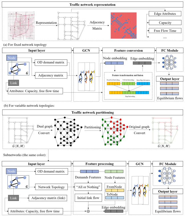
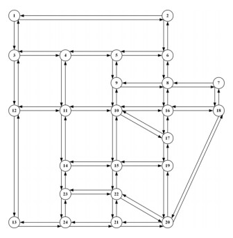
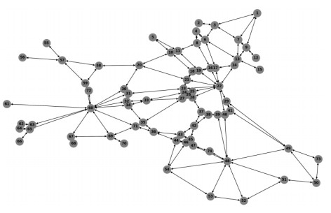
The traffic assignment problem (TAP) is essential to efficient road network operation and significantly influences urban mobility and development. Traditional optimization algorithms typically rely on strict assumptions and iterative optimization methods, making them computationally intensive and inflexible. Deep learning methods, conversely, offer a promising alternative by effectively capturing heterogeneous and nonlinear traffic flow characteristics from diverse datasets. This study introduced a graph convolutional network (GCN)-based framework for the user equilibrium traffic assignment problem (UE-TAP). Specifically, the proposed GCN model learned the implicit relationships between origin-destination (OD) demand matrices and the resulting equilibrium traffic flows, providing efficient and reliable traffic flow estimations without iterative computations. Furthermore, to accommodate variations in network topology, an innovative deep learning approach based on network partitioning and subgraph training was introduced, significantly enhancing the scalability and adaptability of the model. Numerical experiments conducted on the Sioux-Falls and Eastern Massachusetts networks demonstrated that the proposed model achieved robust and high-accuracy estimations across diverse scenarios. In fixed-topology scenarios with random variations in OD demands and link capacities, the proposed model achieved $ {R}^{2} $ of approximately 0.90. Even in scenarios with random link failures coupled with varying OD demands and capacities, the model maintained $ {R}^{2} $ of around 0.84. Overall, the proposed methodology represented a significant advancement in solving UE-TAP, particularly in dynamic environments with evolving road network structures.
Citation: Xin Liu, Yuan Zhang, Kai Zhang, Qixiu Cheng, Jiping Xing, Zhiyuan Liu. A scalable learning approach for user equilibrium traffic assignment problem using graph convolutional networks[J]. Electronic Research Archive, 2025, 33(5): 3246-3270. doi: 10.3934/era.2025143
The traffic assignment problem (TAP) is essential to efficient road network operation and significantly influences urban mobility and development. Traditional optimization algorithms typically rely on strict assumptions and iterative optimization methods, making them computationally intensive and inflexible. Deep learning methods, conversely, offer a promising alternative by effectively capturing heterogeneous and nonlinear traffic flow characteristics from diverse datasets. This study introduced a graph convolutional network (GCN)-based framework for the user equilibrium traffic assignment problem (UE-TAP). Specifically, the proposed GCN model learned the implicit relationships between origin-destination (OD) demand matrices and the resulting equilibrium traffic flows, providing efficient and reliable traffic flow estimations without iterative computations. Furthermore, to accommodate variations in network topology, an innovative deep learning approach based on network partitioning and subgraph training was introduced, significantly enhancing the scalability and adaptability of the model. Numerical experiments conducted on the Sioux-Falls and Eastern Massachusetts networks demonstrated that the proposed model achieved robust and high-accuracy estimations across diverse scenarios. In fixed-topology scenarios with random variations in OD demands and link capacities, the proposed model achieved $ {R}^{2} $ of approximately 0.90. Even in scenarios with random link failures coupled with varying OD demands and capacities, the model maintained $ {R}^{2} $ of around 0.84. Overall, the proposed methodology represented a significant advancement in solving UE-TAP, particularly in dynamic environments with evolving road network structures.

| [1] |
J. Xing, R. Liu, K. Anish, Z. Liu, A customized data fusion tensor approach for interval-wise missing network volume imputation, IEEE Trans. Intell. Transp. Syst., 24 (2023), 12107–12122. https://doi.org/10.1109/TITS.2023.3289193. doi: 10.1109/TITS.2023.3289193

|
| [2] | J. Xing, R. Liu, Y. Zhang, C. F. Choudhury, X. Fu, Q. Cheng, Urban network-wide traffic volume estimation under sparse deployment of detectors, Transportmetrica A: Transp. Sci., 20 (2024). https://doi.org/10.1080/23249935.2023.2197511. |
| [3] |
J. Xing, W. Wu, Q. Cheng, R. Liu, Traffic state estimation of urban road networks by multi-source data fusion: Review and new insights, Physica A Stat. Mech. Appl., 595 (2022), 127079. https://doi.org/10.1016/j.physa.2022.127079. doi: 10.1016/j.physa.2022.127079
|
| [4] |
Y. Jiang, O. A. Nielsen, Urban multimodal traffic assignment, Multimodal Transp., 1 (2022), 100027. https://doi.org/10.1016/j.multra.2022.100027. doi: 10.1016/j.multra.2022.100027
|
| [5] |
D. Huang, J. Zhang, Z. Liu, A robust coordinated charging scheduling approach for hybrid electric bus charging systems, Transp. Res. Part D: Transp. Environ., 125 (2023), 103955. https://doi.org/10.1016/j.trd.2023.103955. doi: 10.1016/j.trd.2023.103955
|
| [6] |
Z. Zhou, Z. Gu, X. Qu, P. Liu, Z. Liu, W. Yu, Urban mobility foundation model: A literature review and hierarchical perspective, Transp. Res. Part E: Logist. Transp. Rev., 192 (2024), 103795. https://doi.org/10.1016/j.tre.2024.103795. doi: 10.1016/j.tre.2024.103795
|
| [7] |
J. Huo, Z. Liu, J. Chen, Q. Cheng, Q. Meng, Bayesian optimization for congestion pricing problems: A general framework and its instability, Transp. Res. Part B: Methodol., 169 (2023), 1–28. https://doi.org/10.1016/j.trb.2023.01.003. doi: 10.1016/j.trb.2023.01.003
|
| [8] |
D. Huang, Y. Gu, S. Wang, Z. Liu, W. Zhang, A two-phase optimization model for the demand-responsive customized bus network design, Transp. Res. Part C: Emerg. Technol., 111 (2020), 1–21. https://doi.org/10.1016/j.trc.2019.12.004. doi: 10.1016/j.trc.2019.12.004
|
| [9] | D. Wang, F. X. Liao, Formulation and solution for calibrating boundedly rational activity-travel assignment: An exploratory study, Commun. Transp. Res., 3 (2023). https://doi.org/10.1016/j.commtr.2023.100092. |
| [10] |
C. Liu, Z. Wang, Z. Liu, K. Huang, Multi-agent reinforcement learning framework for addressing demand-supply imbalance of shared autonomous electric vehicle, Transp. Res. Part E: Logist. Transp. Rev., 197 (2025), 104062. https://doi.org/10.1016/j.tre.2025.104062. doi: 10.1016/j.tre.2025.104062
|
| [11] |
D. Huang, Z. Liu, P. Liu, J. Chen, Optimal transit fare and service frequency of a nonlinear origin-destination based fare structure, Transp. Res. Part E: Logist. Transp. Rev., 96 (2016), 1–19. https://doi.org/10.1016/j.tre.2016.10.004. doi: 10.1016/j.tre.2016.10.004
|
| [12] |
Z. Gu, Y. Li, M. Saberi, T. H. Rashidi, Z. Liu, Macroscopic parking dynamics and equitable pricing: Integrating trip-based modeling with simulation-based robust optimization, Transp. Res. Part B: Methodol., 173 (2023), 354–381. https://doi.org/10.1016/j.trb.2023.05.011. doi: 10.1016/j.trb.2023.05.011
|
| [13] |
Z. Liu, X. Chen, Q. Meng, I. Kim, Remote park-and-ride network equilibrium model and its applications, Transp. Res. Part B: Methodol., 117 (2018), 37–62. https://doi.org/10.1016/j.trb.2018.08.004. doi: 10.1016/j.trb.2018.08.004
|
| [14] | Y. Gu, A. Chen, S. Jang, S. Kitthamkesorn, A binary choice model for adoption of an emerging travel mode with unique service features, Commun. Transp. Res., 4 (2024). https://doi.org/10.1016/j.commtr.2024.100121. |
| [15] | J. G. Wardrop, Road paper. some theoretical aspects of road traffic research, 1 (1952), 325–362. https://doi.org/10.1680/ipeds.1952.11259. |
| [16] | M. Beckmann, C. B. McGuire, C. B. Winsten, Studies in the Economics of Transportation, 1956. |
| [17] |
M. Frank, P. Wolfe, An algorithm for quadratic programming, Naval Res. Logist. Q., 3 (1956), 95–110. https://doi.org/10.1002/nav.3800030109. doi: 10.1002/nav.3800030109
|
| [18] |
M. Florian, J. Guálat, H. Spiess, An efficient implementation of the "Partan" variant of the linear approximation method for the network equilibrium problem, Networks, 17 (1987), 319–339. https://doi.org/10.1002/net.3230170307. doi: 10.1002/net.3230170307
|
| [19] |
S. Lawphongpanich, D. W. Hearn, Simplical decomposition of the asymmetric traffic assignment problem, Transp. Res. Part B: Methodol., 18 (1984), 123–133. https://doi.org/10.1016/0191-2615(84)90026-2. doi: 10.1016/0191-2615(84)90026-2
|
| [20] |
M. Mitradjieva, P. O. Lindberg, The stiff is moving—conjugate direction Frank-Wolfe Methods with applications to traffic assignment, Transp. Sci., 47 (2013), 280–293. https://doi.org/10.1287/trsc.1120.0409. doi: 10.1287/trsc.1120.0409
|
| [21] |
H. Bar-Gera, Origin-based algorithm for the traffic assignment problem, Transp. Sci., 36 (2002), 398–417. https://doi.org/10.1287/trsc.36.4.398.549. doi: 10.1287/trsc.36.4.398.549
|
| [22] |
Y. M. Nie, A class of bush-based algorithms for the traffic assignment problem, Transp. Res. Part B: Methodol., 44 (2010), 73–89. https://doi.org/10.1016/j.trb.2009.06.005. doi: 10.1016/j.trb.2009.06.005
|
| [23] | J. Xie, C. Xie, Origin-based algorithms for traffic assignment: algorithmic structure, complexity analysis, and convergence performance, Transp. Res. Rec., 2498 (2015), 46–55. https://doi.org/10.3141/2498-06. |
| [24] | R. Jayakrishnan, W. T. Tsai, J. N. Prashker, S. Rajadhyaksha, A faster path-based algorithm for traffic assignment, in Transportation Research Board 73rd Annual Meeting, 1994. |
| [25] |
T. Larsson, M. Patriksson, Simplicial decomposition with disaggregated representation for the traffic assignment problem, Transp. Sci., 26 (1992), 4–17. https://doi.org/10.1287/trsc.26.1.4. doi: 10.1287/trsc.26.1.4
|
| [26] |
J. Xie, Y. Nie, X. Liu, A greedy path-based algorithm for traffic assignment, Transp. Res. Rec., 2672 (2018), 36–44. https://doi.org/10.1177/0361198118774236. doi: 10.1177/0361198118774236
|
| [27] |
K. Zhang, H. Zhang, Y. Dong, Y. Wu, X. Chen, An ADMM-based parallel algorithm for solving traffic assignment problem with elastic demand, Commun. Transp. Res., 3 (2023), 100108. https://doi.org/10.1016/j.commtr.2023.100108. doi: 10.1016/j.commtr.2023.100108
|
| [28] |
K. Zhang, H. Zhang, Q. Cheng, X. Chen, Z. Wang, Z. Liu, A customized two-stage parallel computing algorithm for solving the combined modal split and traffic assignment problem, Comput. Oper. Res., 154 (2023), 106193. https://doi.org/10.1016/j.cor.2023.106193. doi: 10.1016/j.cor.2023.106193
|
| [29] |
X. Chen, Z. Liu, K. Zhang, Z. Wang, A parallel computing approach to solve traffic assignment using path-based gradient projection algorithm, Transp. Res. Part C: Emerg. Technol., 120 (2020), 102809. https://doi.org/10.1016/j.trc.2020.102809. doi: 10.1016/j.trc.2020.102809
|
| [30] |
H. Zhang, Z. Liu, J. Wang, Y. Wu, A novel flow update policy in solving traffic assignment problems: Successive over relaxation iteration method, Transp. Res. Part E: Logist. Transp. Rev., 174 (2023), 103111. https://doi.org/10.1016/j.tre.2023.103111. doi: 10.1016/j.tre.2023.103111
|
| [31] |
Z. Liu, X. Chen, J. Hu, S. Wang, K. Zhang, H. Zhang, An alternating direction method of multipliers for solving user equilibrium problem, Eur. J. Oper. Res., 310 (2023), 1072–1084. https://doi.org/10.1016/j.ejor.2023.04.008. doi: 10.1016/j.ejor.2023.04.008
|
| [32] |
M. Veres, M. Moussa, Deep learning for intelligent transportation systems: A survey of emerging trends, IEEE Trans. Intell. Transp. Syst., 21 (2019), 3152–3168. https://doi.org/10.1109/TITS.2019.2929020. doi: 10.1109/TITS.2019.2929020
|
| [33] |
H. Nguyen, L. M. Kieu, T. Wen, C. Cai, Deep learning methods in transportation domain: a review, IET Intell. Transp. Syst., 12 (2018), 998–1004. https://doi.org/10.1049/iet-its.2018.0064. doi: 10.1049/iet-its.2018.0064
|
| [34] |
Z. Zhao, W. Chen, X. Wu, P. C. Chen, J. Liu, LSTM network: a deep learning approach for short‐term traffic forecast, IET Intell. Transp. Syst., 11 (2017), 68–75. https://doi.org/10.1049/iet-its.2016.0208. doi: 10.1049/iet-its.2016.0208
|
| [35] |
Y. Lv, Y. Duan, W. Kang, Z. Li, F. Y. Wang, Traffic flow prediction with big data: A deep learning approach, IEEE Trans. Intell. Transp. Syst., 16 (2014), 865–873. https://doi.org/10.1109/TITS.2014.2345663. doi: 10.1109/TITS.2014.2345663
|
| [36] | J. Xing, X. Jiang, Y. Yuan, W. Liu, Incorporating mobile phone data-based travel mobility analysis of metro ridership in aboveground and underground layers, Electron. Res. Arch., 32 (2024). https://doi.org/10.3934/era.2024202. |
| [37] |
A. Nigam, S. Srivastava, Hybrid deep learning models for traffic stream variables prediction during rainfall, Multimodal Transp., 2 (2023), 100052. https://doi.org/10.1016/j.multra.2022.100052. doi: 10.1016/j.multra.2022.100052
|
| [38] |
Y. Liu, Z. Liu, R. Jia, DeepPF: A deep learning based architecture for metro passenger flow prediction, Transp. Res. Part C: Emerg. Technol., 101 (2019), 18–34. https://doi.org/10.1016/j.trc.2019.01.027. doi: 10.1016/j.trc.2019.01.027
|
| [39] |
D. Huang, J. Zhang, Z. Liu, Y. He, P. Liu, A novel ranking method based on semi-SPO for battery swapping allocation optimization in a hybrid electric transit system, Transp. Res. Part E: Logist. Transp. Rev., 188 (2024), 103611. https://doi.org/10.1016/j.tre.2024.103611. doi: 10.1016/j.tre.2024.103611
|
| [40] |
J. Zhang, D. Huang, Z. Liu, Y. Zheng, Y. Han, P. Liu, et al., A data-driven optimization-based approach for freeway traffic state estimation based on heterogeneous sensor data fusion, Transp. Res. Part E: Logist. Transp. Rev., 189 (2024), 103656. https://doi.org/10.1016/j.tre.2024.103656. doi: 10.1016/j.tre.2024.103656
|
| [41] |
Z. Gu, X. Yang, Q. Zhang, W. Yu, Z. Liu, TERL: Two-stage ensemble reinforcement learning paradigm for large-scale decentralized decision making in transportation simulation, IEEE Trans. Knowl. Data Eng., 35 (2023), 13043–13054. https://doi.org/10.1109/TKDE.2023.3272688. doi: 10.1109/TKDE.2023.3272688
|
| [42] |
Z. Gu, Y. Wang, W. Ma, Z. Liu, A joint travel mode and departure time choice model in dynamic multimodal transportation networks based on deep reinforcement learning, Multimodal Transp., 3 (2024), 100137. https://doi.org/10.1016/j.multra.2024.100137. doi: 10.1016/j.multra.2024.100137
|
| [43] |
R. Rahman, S. Hasan, Data-driven traffic assignment: A novel approach for learning traffic flow patterns using graph convolutional neural network, Data Sci. Transp., 5 (2023), 11. https://doi.org/10.1007/s42421-023-00073-y. doi: 10.1007/s42421-023-00073-y
|
| [44] |
P. Guarda, M. Battifarano, S. Qian, Estimating network flow and travel behavior using day-to-day system-level data: A computational graph approach, Transp. Res. Part C: Emerg. Technol., 158 (2024), 104409. https://doi.org/10.1016/j.trc.2023.104409. doi: 10.1016/j.trc.2023.104409
|
| [45] |
B. Sifringer, V. Lurkin, A. Alahi, Enhancing discrete choice models with representation learning, Transp. Res. Part B: Methodol., 140 (2020), 236–261. https://doi.org/10.1016/j.trb.2020.08.006. doi: 10.1016/j.trb.2020.08.006
|
| [46] | Z. Fang, Q. Cheng, Z. Liu, Y. Liu, A deep learning approach for the traffic assignment problem, in Transportation Research Board 98th Annual Meeting, 2019. |
| [47] |
Z. Liu, Y. Yin, F. Bai, D. K. Grimm, End-to-end learning of user equilibrium with implicit neural networks, Transp. Res. Part C: Emerg. Technol., 150 (2023), 104085. https://doi.org/10.1016/j.trc.2023.104085. doi: 10.1016/j.trc.2023.104085
|
| [48] | Z. Liu, Y. Yin, End-to-end learning of user equilibrium: Expressivity, generalization, and optimization, Transp. Sci., 2025. https://doi.org/10.1287/trsc.2023.0489. |
| [49] |
W. Fan, Z. Tang, P. Ye, F. Xiao, J. Zhang, Deep learning-based dynamic traffic assignment with incomplete origin–destination data, Transp. Res. Rec., 2677 (2023), 1340–1356. https://doi.org/10.1177/03611981221123805. doi: 10.1177/03611981221123805
|
| [50] |
X. Hu, C. Xie, Use of graph attention networks for traffic assignment in a large number of network scenarios, Transp. Res. Part C: Emerg. Technol., 171 (2025), 104997. https://doi.org/10.1016/j.trc.2025.104997. doi: 10.1016/j.trc.2025.104997
|
| [51] | T. N. Kipf, M. Welling, Semi-supervised classification with graph convolutional networks, in International Conference on Learning Representations, 2017. |
| [52] |
M. R. McCord, Urban transportation networks: Equilibrium analysis with mathematical programming methods, Transp. Res. Part A: Policy Pract., 21 (1987), 481–484. https://doi.org/10.1016/0191-2607(87)90038-0. doi: 10.1016/0191-2607(87)90038-0
|
| [53] | K. Lab, METIS-Serial Graph Partitioning and Fill-reducing Matrix Ordering, 2016. |
Figures(18) / Tables(11)
Xin Liu, Yuan Zhang, Kai Zhang, Qixiu Cheng, Jiping Xing, Zhiyuan Liu. A scalable learning approach for user equilibrium traffic assignment problem using graph convolutional networks[J]. Electronic Research Archive, 2025, 33(5): 3246-3270. doi: 10.3934/era.2025143


 DownLoad: