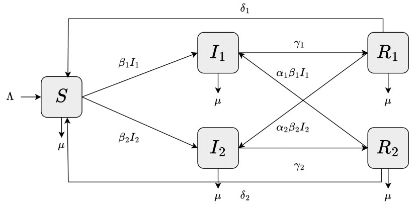
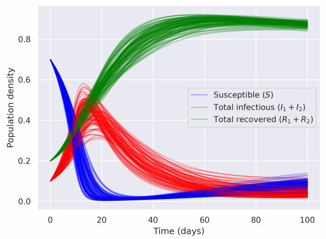
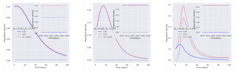
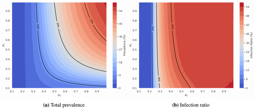
In this study, we developed a mathematical framework, based on the SIR model, to study the dynamics of two competing virus variants with different characteristics of transmissibility, immune escape, and cross-immunity. The model includes variant-specific transmission and recovery rates and enables flexible parameterization of partial and waning cross-immunity. We conducted stability and bifurcation analyses and numerical simulations to explore the conditions of coexistence, dominance, and extinction of the variants, studying variations in epidemiological parameters that affect endemic prevalence and infection ratios. Our results indicated that transmission rates, levels of cross-immunity, and immunity waning rates are critical in determining disease outcomes, which influence variant prevalence and competitive dynamics. The sensitivity analysis provided the relative importance of these parameters and provided valuable insight into designing intervention strategies. This work contributes to furthering our understanding of multi-variant epidemic dynamics and lays the bedrock for tackling complex interactions involving arising virus variants, finding applications in real-world public health planning.
Citation: Shirali Kadyrov, Farkhod Haydarov, Khudoyor Mamayusupov, Komil Mustayev. Endemic coexistence and competition of virus variants under partial cross-immunity[J]. Electronic Research Archive, 2025, 33(2): 1120-1143. doi: 10.3934/era.2025050
In this study, we developed a mathematical framework, based on the SIR model, to study the dynamics of two competing virus variants with different characteristics of transmissibility, immune escape, and cross-immunity. The model includes variant-specific transmission and recovery rates and enables flexible parameterization of partial and waning cross-immunity. We conducted stability and bifurcation analyses and numerical simulations to explore the conditions of coexistence, dominance, and extinction of the variants, studying variations in epidemiological parameters that affect endemic prevalence and infection ratios. Our results indicated that transmission rates, levels of cross-immunity, and immunity waning rates are critical in determining disease outcomes, which influence variant prevalence and competitive dynamics. The sensitivity analysis provided the relative importance of these parameters and provided valuable insight into designing intervention strategies. This work contributes to furthering our understanding of multi-variant epidemic dynamics and lays the bedrock for tackling complex interactions involving arising virus variants, finding applications in real-world public health planning.

| [1] |
A. Elaiw, E. Almohaimeed, A. Hobiny, Modeling the co-infection of HTLV-2 and HIV-1 in vivo, Electron. Res. Arch., 32 (2024), 6032–6071. https://doi.org/10.3934/era.2024280 doi: 10.3934/era.2024280

|
| [2] |
W. O. Kermack, A. G. McKendrick, A contribution to the mathematical theory of epidemics, Proc. R. Soc. London, Ser. A, 115 (1927), 700–721. https://doi.org/10.1098/rspa.1927.0118 doi: 10.1098/rspa.1927.0118
|
| [3] |
V. Andreasen, J. Lin, S. A. Levin, The dynamics of cocirculating influenza strains conferring partial cross-immunity, J. Math. Biol., 35 (1997), 825–842. https://doi.org/10.1007/s002850050079 doi: 10.1007/s002850050079
|
| [4] |
M. Kamo, A. Sasaki, The effect of cross-immunity and seasonal forcing in a multi-strain epidemic model, Physica D: Nonlinear Phenom., 165 (2002), 228–241. https://doi.org/10.1016/S0167-2789(02)00389-5 doi: 10.1016/S0167-2789(02)00389-5
|
| [5] |
S. M. Garba, A. B. Gumel, Effect of cross-immunity on the transmission dynamics of two strains of dengue, Int. J. Comput. Math., 87 (2010), 2361–2384. https://doi.org/10.1080/00207160802660608 doi: 10.1080/00207160802660608
|
| [6] |
K. Sneppen, A. Trusina, M. H. Jensen, S. Bornholdt, A minimal model for multiple epidemics and immunity spreading, PloS One, 5 (2010), e13326. https://doi.org/10.1371/journal.pone.0013326 doi: 10.1371/journal.pone.0013326
|
| [7] |
M. D. Johnston, B. Pell, D. Rubel, A two-strain model of infectious disease spread with asymmetric temporary immunity periods and partial cross-immunity, Math. Biosci. Eng., 20 (2023), 16083–16113, https://doi.org/10.3934/mbe.2023718 doi: 10.3934/mbe.2023718
|
| [8] | B. Pell, S. Brozak, T. Phan, F. Wu, Y. Kuang, The emergence of a virus variant: Dynamics of a competition model with cross-immunity time-delay validated by wastewater surveillance data for COVID-19, J. Math. Biol., 86 (2023). https://doi.org/10.1007/s00285-023-01900-0 |
| [9] |
M. Ogura, V. M. Preciado, Epidemic processes over adaptive state-dependent networks, Phys. Rev. E, 93 (2016), 062316. https://doi.org/10.1103/PhysRevE.93.062316 doi: 10.1103/PhysRevE.93.062316
|
| [10] |
O. M. Otunuga, Analysis of multi-strain infection of vaccinated and recovered population through epidemic model: Application to COVID-19, PloS One, 17 (2022), e0271446. https://doi.org/10.1371/journal.pone.0271446 doi: 10.1371/journal.pone.0271446
|
| [11] |
D. A. B. Lombana, L. Zino, S. Butail, E. Caroppo, Z. P. Jiang, A. Rizzo, et al., Activity-driven network modeling and control of the spread of two concurrent epidemic strains, Appl. Network Sci., 7 (2022), 66. https://doi.org/10.1007/s41109-022-00507-6 doi: 10.1007/s41109-022-00507-6
|
| [12] | K. Olumoyin, A. Khaliq, Multi-variant COVID-19 model with heterogeneous transmission rates using deep neural networks, preprint, arXiv: 2205.06834. |
| [13] |
N. Bessonov, D. Neverova, V. Popov, V. Volpert, Emergence and competition of virus variants in respiratory viral infections, Front. Immunol., 13 (2023), 945228. https://doi.org/10.3389/fimmu.2022.945228 doi: 10.3389/fimmu.2022.945228
|
| [14] |
N. G. Reich, S. Shrestha, A. A. King, P. Rohani, J. Lessler, S. Kalayanarooj, et al., Interactions between serotypes of dengue highlight epidemiological impact of cross-immunity, J. R. Soc. Interface, 10 (2013), 20130414. https://doi.org/10.1098/rsif.2013.0414 doi: 10.1098/rsif.2013.0414
|
| [15] |
N. M. Ferguson, A. P. Galvani, R. M. Bush, Ecological and immunological determinants of influenza evolution, Nature, 422 (2003), 428–433. https://doi.org/10.1038/nature01509 doi: 10.1038/nature01509
|
| [16] |
V. Andreasen, Epidemics in competition: Partial cross-immunity, Bull. Math. Biol., 80 (2018), 2957–2977. https://doi.org/10.1007/s11538-018-0495-2 doi: 10.1007/s11538-018-0495-2
|
| [17] |
R. Sachak-Patwa, H. M. Byrne, R. N. Thompson, Accounting for cross-immunity can improve forecast accuracy during influenza epidemics, Epidemics, 34 (2021), 100432. https://doi.org/10.1016/j.epidem.2020.100432 doi: 10.1016/j.epidem.2020.100432
|
| [18] |
I. Atienza-Diez, L. F. Seoane, Long-and short-term effects of cross-immunity in epidemic dynamics, Chaos, Solitons & Fractals, 174 (2023), 113800. https://doi.org/10.1016/j.chaos.2023.113800 doi: 10.1016/j.chaos.2023.113800
|
| [19] |
K. Chung, R. Lui, Dynamics of two-strain influenza model with cross-immunity and no quarantine class, J. Math. Biol., 73 (2016), 1467–1489. https://doi.org/10.1007/s00285-016-1000-x doi: 10.1007/s00285-016-1000-x
|
| [20] | R. Niu, Y. C. Chan, S. Liu, E. W. Wong, M. A. van Wyk, Stability analysis of an epidemic model with two competing variants and cross-infections, preprint. https://doi.org/10.21203/rs.3.rs-3264948/v1 |
| [21] |
S. Ojosnegros, E. Delgado-Eckert, N. Beerenwinkel, Competition–colonization trade-off promotes coexistence of low-virulence viral strains, J. R. Soc. Interface, 9 (2012), 2244–2254. https://doi.org/10.1098/rsif.2012.0160 doi: 10.1098/rsif.2012.0160
|
| [22] |
E. W. Seabloom, E. T. Borer, K. Gross, A. E. Kendig, C. Lacroix, C. E. Mitchell, et al., The community ecology of pathogens: Coinfection, coexistence and community composition, Ecol. Lett., 18 (2015), 401–415. https://doi.org/10.1111/ele.12418 doi: 10.1111/ele.12418
|
| [23] |
E. Gjini, C. Valente, R. Sa-Leao, M. G. M. Gomes, How direct competition shapes coexistence and vaccine effects in multi-strain pathogen systems, J. Theor. Biol., 388 (2016), 50–60. https://doi.org/10.1016/j.jtbi.2015.09.031 doi: 10.1016/j.jtbi.2015.09.031
|
| [24] |
A. S. Ackleh, K. Deng, Y. Wu, Competitive exclusion and coexistence in a two-strain pathogen model with diffusion, Math. Biosci. Eng., 13 (2015), 1–18. https://doi.org/10.3934/mbe.2016.13.1 doi: 10.3934/mbe.2016.13.1
|
| [25] |
J. Amador, D. Armesto, A. Gómez-Corral, Extreme values in sir epidemic models with two strains and cross-immunity, Math. Biosci. Eng., 16 (2019), 1992–2022. https://doi.org/10.3934/mbe.2019098 doi: 10.3934/mbe.2019098
|
| [26] |
L. F. Jover, M. H. Cortez, J. S. Weitz, Mechanisms of multi-strain coexistence in host–phage systems with nested infection networks, J. Theor. Biol., 332 (2013), 65–77. https://doi.org/10.1016/j.jtbi.2013.04.011 doi: 10.1016/j.jtbi.2013.04.011
|
| [27] |
R. Rifhat, K. Wang, L. Wang, T. Zeng, Z. Teng, Global stability of multi-group seiqr epidemic models with stochastic perturbation in computer network, Electron. Res. Arch., 31 (2023), 4155–4184. https://doi.org/10.3934/era.2023212 doi: 10.3934/era.2023212
|
| [28] |
H. G. Anderson, G. P. Takacs, D. C. Harris, Y. Kuang, J. K. Harrison, T. L. Stepien, Global stability and parameter analysis reinforce therapeutic targets of PD-l1-PD-1 and MDSCs for glioblastoma, J. Math. Biol., 88 (2024), 10. https://doi.org/10.1007/s00285-023-02027-y doi: 10.1007/s00285-023-02027-y
|
| [29] | F. Brauer, J. A. Nohel, The Qualitative Theory of Ordinary Differential Equations: An Introduction, Courier Corporation, 1989. |
| [30] |
A. Lajmanovich, J. A. Yorke, A deterministic model for gonorrhea in a nonhomogeneous population, Math. Biosci., 28 (1976), 221–236. https://doi.org/10.1016/0025-5564(76)90125-5 doi: 10.1016/0025-5564(76)90125-5
|
| [31] |
C. N. Ngonghala, H. B. Taboe, S. Safdar, A. B. Gumel, Unraveling the dynamics of the omicron and delta variants of the 2019 coronavirus in the presence of vaccination, mask usage, and antiviral treatment, Appl. Math. Modell., 114 (2023), 447–465. https://doi.org/10.1016/j.apm.2022.09.017 doi: 10.1016/j.apm.2022.09.017
|
| [32] |
C. Menni, A. M. Valdes, L. Polidori, M. Antonelli, S. Penamakuri, A. Nogal, et al., Symptom prevalence, duration, and risk of hospital admission in individuals infected with SARS-COV-2 during periods of omicron and delta variant dominance: A prospective observational study from the zoe covid study, The Lancet, 399 (2022), 1618–1624. https://doi.org/10.1016/S0140-6736(22)00327-0 doi: 10.1016/S0140-6736(22)00327-0
|
| [33] |
S. Liossi, E. Tsiambas, S. Maipas, E. Papageorgiou, A. Lazaris, N. Kavantzas, Mathematical modeling for delta and omicron variant of SARS-COV-2 transmission dynamics in greece, Infect. Dis. Modell., 8 (2023), 794–805. https://doi.org/10.1016/j.idm.2023.07.002 doi: 10.1016/j.idm.2023.07.002
|
| [34] | C. Cassata, How long does immunity last after COVID-19? What we know, Healthline, 2021 (2021). |
| [35] |
Y. Liu, J. Rocklöv, The reproductive number of the delta variant of SARS-COV-2 is far higher compared to the ancestral SARS-COV-2 virus, J. Travel Med., 28 (2021), taab124. https://doi.org/10.1093/jtm/taab124 doi: 10.1093/jtm/taab124
|
| [36] |
Y. Liu, J. Rocklöv, The effective reproductive number of the omicron variant of SARS-COV-2 is several times relative to delta, J. Travel Med., 29 (2022), taac037. https://doi.org/10.1093/jtm/taac037 doi: 10.1093/jtm/taac037
|
| [37] |
L. Hanum, D. Ertiningsih, N. Susyanto, Sensitivity analysis unveils the interplay of drug-sensitive and drug-resistant glioma cells: Implications of chemotherapy and anti-angiogenic therapy, Electron. Res. Arch., 32 (2024), 72–89. https://doi.org/10.3934/era.2024004 doi: 10.3934/era.2024004
|
Figures(8) / Tables(3)
Shirali Kadyrov, Farkhod Haydarov, Khudoyor Mamayusupov, Komil Mustayev. Endemic coexistence and competition of virus variants under partial cross-immunity[J]. Electronic Research Archive, 2025, 33(2): 1120-1143. doi: 10.3934/era.2025050


 DownLoad: