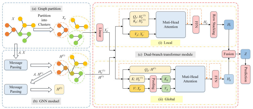
As an emerging architecture, graph Transformers (GTs) have demonstrated significant potential in various graph-related tasks. Existing GTs are mainly oriented to graph-level tasks and have proved their advantages, but they do not perform well in node classification tasks. This mainly comes from two aspects: (1) The global attention mechanism causes the computational complexity to grow quadratically with the number of nodes, resulting in substantial resource demands, especially on large-scale graphs; (2) a large number of long-distance irrelevant nodes disperse the attention weights and weaken the focus on local neighborhoods. To address these issues, we proposed a new model, dual-branch graph Transformer (DCAFormer). The model divided the graph into clusters with the same number of nodes by a graph partitioning algorithm to reduce the number of input nodes. Subsequently, the original graph was processed by graph neural network (GNN) to obtain outputs containing structural information. Next, we adopted a dual-branch architecture: The local branch (intracluster Transformer) captured local information within each cluster, reducing the impact of long-distance irrelevant nodes on attention; the global branch (intercluster Transformer) captured global interactions across clusters. Meanwhile, we designed a hybrid feature mechanism that integrated original features with GNN outputs and separately optimized the construction of the query ($ Q $), key ($ K $), and value ($ V $) matrices of the intracluster and intercluster Transformers in order to adapt to the different modeling requirements of two branches. We conducted extensive experiments on 8 benchmark node classification datasets, and the results showed that DCAFormer outperformed existing GTs and mainstream GNNs.
Citation: Yong Zhang, Jingjing Song, Eric C.C. Tsang, Yingxing Yu. Dual-branch graph Transformer for node classification[J]. Electronic Research Archive, 2025, 33(2): 1093-1119. doi: 10.3934/era.2025049
As an emerging architecture, graph Transformers (GTs) have demonstrated significant potential in various graph-related tasks. Existing GTs are mainly oriented to graph-level tasks and have proved their advantages, but they do not perform well in node classification tasks. This mainly comes from two aspects: (1) The global attention mechanism causes the computational complexity to grow quadratically with the number of nodes, resulting in substantial resource demands, especially on large-scale graphs; (2) a large number of long-distance irrelevant nodes disperse the attention weights and weaken the focus on local neighborhoods. To address these issues, we proposed a new model, dual-branch graph Transformer (DCAFormer). The model divided the graph into clusters with the same number of nodes by a graph partitioning algorithm to reduce the number of input nodes. Subsequently, the original graph was processed by graph neural network (GNN) to obtain outputs containing structural information. Next, we adopted a dual-branch architecture: The local branch (intracluster Transformer) captured local information within each cluster, reducing the impact of long-distance irrelevant nodes on attention; the global branch (intercluster Transformer) captured global interactions across clusters. Meanwhile, we designed a hybrid feature mechanism that integrated original features with GNN outputs and separately optimized the construction of the query ($ Q $), key ($ K $), and value ($ V $) matrices of the intracluster and intercluster Transformers in order to adapt to the different modeling requirements of two branches. We conducted extensive experiments on 8 benchmark node classification datasets, and the results showed that DCAFormer outperformed existing GTs and mainstream GNNs.

| [1] | W. Q. Fan, Y. Ma, Q. Li, Y. He, E. Zhao, J. L. Tang, et al., Graph neural networks for social recommendation, in Proceedings of the 2019 World Wide Web Conference, (2019), 417–426. https://doi.org/10.1145/3308558.3313488 |
| [2] | N. Xu, P. H. Wang, L. Chen, J. Tao, J. Z. Zhao, MR-GNN: Multi-resolution and dual graph neural network for predicting structured entity interactions, in Proceedings of the 28th International Joint Conference on Artificial Intelligence, (2019), 3968–3974. https://doi.org/10.24963/ijcai.2019/551 |
| [3] | P. Y. Zhang, Y. C. Yan, X. Zhang, L. C. Li, S. Z. Wang, F. R. Huang, et al., TransGNN: Harnessing the collaborative power of transformers and graph neural networks for recommender systems, in Proceedings of the 47th International ACM SIGIR Conference on Research and Development in Information Retrieval, (2024), 1285–1295. https://doi.org/10.1145/3626772.3657721 |
| [4] |
S. X. Ji, S. R. Pan, E. Cambria, P. Marttinen, S. Y. Philip, A survey on knowledge graphs: Representation, acquisition, and applications, IEEE Trans. Neural Networks Learn. Syst., 33 (2021), 494–514. https://doi.org/10.1109/TNNLS.2021.3070843 doi: 10.1109/TNNLS.2021.3070843

|
| [5] | T. N. Kipf, M. Welling, Semi-supervised classification with graph convolutional networks, preprint, arXiv: 1609.02907. https://doi.org/10.48550/arXiv.1609.02907 |
| [6] | P. Veličković, G. Cucurull, A. Casanova, A. Romero, P. Liò, Y. Bengio, Graph attention networks, preprint, arXiv: 1710.10903. https://doi.org/10.48550/arXiv.1710.10903 |
| [7] | W. Hamilton, Z. T. Ying, J. Leskovec, Inductive representation learning on large graphs, in Advances in Neural Information Processing Systems (eds. I. Guyon, U. Von Luxburg, S. Bengio, H. Wallach, R. Fergus, S. Vishwanathan and R. Garnett), Curran Associates, Inc., 30 (2017). |
| [8] | X. T. Yu, Z. M. Liu, Y. Fang, X. M. Zhang, Learning to count isomorphisms with graph neural networks, in Proceedings of the 37th AAAI Conference on Artificial Intelligence, 37 (2023), 4845–4853. https://doi.org/10.1609/aaai.v37i4.25610 |
| [9] | Q. M. Li, Z. C. Han, X. M. Wu, Deeper insights into graph convolutional networks for semi-supervised learning, in Proceedings of the 32nd AAAI Conference on Artificial Intelligence, 32 (2018), 3538–3545. https://doi.org/10.1609/aaai.v32i1.11604 |
| [10] | J. Topping, F. Di Giovanni, B. P. Chamberlain, X. W. Dong, M. M. Bronstein, Understanding over-squashing and bottlenecks on graphs via curvature, preprint, arXiv: 2111.14522. https://doi.org/10.48550/arXiv.2111.14522 |
| [11] | A. Vaswani, N. Shazeer, N. Parmar, J. Uszkoreit, L. Jones, A. N. Gomez, et al., Attention is all you need, in Advances in Neural Information Processing Systems (eds. I. Guyon, U. Von Luxburg, S. Bengio, H. Wallach, R. Fergus, S. Vishwanathan and R. Garnett), Curran Associates, Inc., 30 (2017). |
| [12] | J. Devlin, M. W. Chang, K. Lee, K. Toutanova, BERT: Pre-training of deep bidirectional transformers for language understanding, in Proceedings of the 2019 Conference of the North American Chapter of the Association for Computational Linguistics: Human Language Technologies, 1 (2019), 4171–4186. https://doi.org/10.18653/v1/N19-1423 |
| [13] | A. Dosovitskiy, L. Beyer, A. Kolesnikov, D. Weissenborn, X. H. Zhai, T. Unterthiner, et al., An image is worth 16$\times$16 words: Transformers for image recognition at scale, in Proceedings of the 9th International Conference on Learning Representations, 2021. |
| [14] | Y. H. Liu, M. Ott, N. Goyal, J. F. Du, M. Joshi, D. Q. Chen, et al., RoBERTa: A robustly optimized bert pretraining approach, preprint, arXiv: 1907.11692. https://doi.org/10.48550/arXiv.1907.11692 |
| [15] | Z. Liu, Y. T. Lin, Y. Cao, H. Hu, Y. X. Wei, Z. Zhang, et al., Swin transformer: Hierarchical vision transformer using shifted windows, in Proceedings of the IEEE/CVF International Conference on Computer Vision, (2021), 10012–10022. https://doi.org/10.1109/ICCV48922.2021.00986 |
| [16] | D. Kreuzer, D. Beaini, W. Hamilton, V. Létourneau, P. Tossou, Rethinking graph transformers with spectral attention, in Advances in Neural Information Processing Systems (eds. M. Ranzato, A. Beygelzimer, Y. Dauphin, P.S. Liang and J. Wortman Vaughan), Curran Associates, Inc., 34 (2021), 21618–21629. |
| [17] |
Y. Ye, S. H. Ji, Sparse graph attention networks, IEEE Trans. Knowl. Data Eng., 35 (2023), 905–916. https://doi.org/10.1109/TKDE.2021.3072345 doi: 10.1109/TKDE.2021.3072345
|
| [18] | C. X. Ying, T. L. Cai, S. J. Luo, S. X. Zheng, G. L. Ke, D. He, et al., Do transformers really perform bad for graph representation?, in Advances in Neural Information Processing Systems (eds. M. Ranzato, A. Beygelzimer, Y. Dauphin, P.S. Liang and J. Wortman Vaughan), Curran Associates, Inc., 34 (2021), 28877–28888. |
| [19] | E. X. Min, R. F. Chen, Y. T. Bian, T. Y. Xu, K. F. Zhao, W. B. Huang, et al., Transformer for graphs: An overview from architecture perspective, preprint, arXiv: 2202.08455. https://doi.org/10.48550/arXiv.2202.08455 |
| [20] | A. Shehzad, F. Xia, S. Abid, C. Y. Peng, S. Yu, D. Y. Zhang, et al., Graph Transformers: A survey, preprint, arXiv: 2407.09777. https://doi.org/10.48550/arXiv.2407.09777 |
| [21] | W. R. Kuang, W. Zhen, Y. L. Li, Z. W. Wei, B. L. Ding, Coarformer: Transformer for large graph via graph coarsening, 2021. Available from: https://openreview.net/forum?id = fkjO_FKVzw |
| [22] | J. N. Zhao, C. Z. Li, Q. L. Wen, Y. Q. Wang, Y. M. Liu, H. Sun, et al., Gophormer: Ego-graph transformer for node classification, preprint, arXiv: 2110.13094. https://doi.org/10.48550/arXiv.2110.13094 |
| [23] | Z. X. Zhang, Q. Liu, Q. Y. Hu, C. K. Lee, Hierarchical graph transformer with adaptive node sampling, in Advances in Neural Information Processing Systems (eds. S. Koyejo, S. Mohamed, A. Agarwal, D. Belgrave, K. Cho and A. Oh), Curran Associates, Inc., 35 (2022), 21171–21183. |
| [24] | C. Liu, Y. B. Zhan, X. Q. Ma, L. Ding, D. P. Tao, J. Wu, et al., Gapformer: Graph transformer with graph pooling for node classification, in Proceedings of the 32nd International Joint Conference on Artificial Intelligence, (2023), 2196–2205. https://doi.org/10.24963/ijcai.2023/244 |
| [25] | J. S. Chen, K. Y. Gao, G. C. Li, K. He, NAGphormer: A tokenized graph transformer for node classification in large graphs, preprint, arXiv: 2206.04910. https://doi.org/10.48550/arXiv.2206.04910 |
| [26] |
K. H. Zhang, D. X. Li, W. H. Luo, W. Q. Ren, Dual attention-in-attention model for joint rain streak and raindrop removal, IEEE Trans. Image Process., 30 (2021), 7608–7619. https://doi.org/10.1109/TIP.2021.3108019 doi: 10.1109/TIP.2021.3108019
|
| [27] |
K. H. Zhang, W. H. Luo, Y. J. Yu, W. Q. Ren, F. Zhao, C. S. Li, et al., Beyond monocular deraining: Parallel stereo deraining network via semantic prior, Int. J. Comput. Vision, 130 (2022), 1754–1769. https://doi.org/10.1007/s11263-022-01620-w doi: 10.1007/s11263-022-01620-w
|
| [28] |
K. H. Zhang, W. Q. Ren, W. H. Luo, W. S. Lai, B. Stenger, M. H. Yang, et al., Deep image deblurring: A survey, Int. J. Comput. Vision, 130 (2022), 2103–2130. https://doi.org/10.1007/s11263-022-01633-5 doi: 10.1007/s11263-022-01633-5
|
| [29] | B. Y. Zhou, Q. Cui, X. S. Wei, Z. M. Chen, BBN: Bilateral-branch network with cumulative learning for long-tailed visual recognition, in Proceedings of the IEEE Computer Society Conference on Computer Vision and Pattern Recognition, CVPR, (2020), 9716–9725. https://doi.org/10.1109/CVPR42600.2020.00974 |
| [30] | T. Wang, Y. Li, B. Y. Kang, J. N. Li, J. H. Liew, S. Tang, et al., The devil is in classification: A simple framework for long-tail instance segmentation, in Computer Vision–ECCV 2020: 16th European Conference, 12359 (2020), 728–744. https://doi.org/10.1007/978-3-030-58568-6_43 |
| [31] | H. Guo, S. Wang, Long-tailed multi-label visual recognition by collaborative training on uniform and re-balanced samplings, in Proceedings of the IEEE Computer Society Conference on Computer Vision and Pattern Recognition, (2021), 15084–15093. https://doi.org/10.1109/CVPR46437.2021.01484 |
| [32] | Y. Zhou, S. Y. Sun, C. Zhang, Y. K. Li, W. L. Ouyang, Exploring the hierarchy in relation labels for scene graph generation, preprint, arXiv: 2009.05834. https://doi.org/10.48550/arXiv.2009.05834 |
| [33] |
C. F. Zheng, L. L. Gao, X. Y. Lyu, P. P. Zeng, A. El Saddik, H. T. Shen, Dual-branch hybrid learning network for unbiased scene graph generation, IEEE Trans. Circuits Syst. Video Technol., 34 (2024), 1743–1756. https://doi.org/10.1109/TCSVT.2023.3297842 doi: 10.1109/TCSVT.2023.3297842
|
| [34] |
G. Karypis, V. Kumar, A fast and high quality multilevel scheme for partitioning irregular graphs, SIAM J. Sci. Comput., 20 (1998), 359–392. https://doi.org/10.1137/S1064827595287997 doi: 10.1137/S1064827595287997
|
| [35] | Y. Rong, Y. T. Bian, T. Y. Xu, W. Y. Xie, Y. Wei, W. B. Huang, et al., Self-supervised graph transformer on large-scale molecular data, in Advances in Neural Information Processing Systems (eds. H. Larochelle, M. Ranzato, R. Hadsell, M.F. Balcan and H. Lin), 33 (2020), 12559–12571. |
| [36] | D. X. Chen, L. O'Bray, K. Borgwardt, Structure-aware transformer for graph representation learning, in Proceedings of the 39th International Conference on Machine Learning, PMLR, 162 (2022), 3469–3489. |
| [37] | J. Klicpera, A. Bojchevski, S. Günnemann, Predict then propagate: Graph neural networks meet personalized pagerank, preprint, arXiv: 1810.05997. https://doi.org/10.48550/arXiv.1810.05997 |
| [38] | L. Page, S. Brin, R. Motwani, T. Winograd, The PageRank Citation Ranking: Bringing Order to the Web., 1998. Available from: http://ilpubs.stanford.edu: 8090/422/ |
| [39] | M. Chen, Z. W. Wei, Z. F. Huang, B. L. Ding, Y. L. Li, Simple and deep graph convolutional networks, in Proceedings of the 37th International Conference on Machine Learning, 119 (2020), 1725–1735. https://doi.org/10.48550/arXiv.2007.02133 |
| [40] | K. M. He, X. Y. Zhang, S. Q. Ren, J. Sun, Deep residual learning for image recognition, in Proceedings of the IEEE Conference on Computer Vision and Pattern Recognition, (2016), 770–778. https://doi.org/10.1109/CVPR.2016.90 |
| [41] | M. Hardt, T. Y. Ma, Identity matters in deep learning, preprint, arXiv: 1611.04231. https://doi.org/10.48550/arXiv.1611.04231 |
| [42] | H. Q. Zeng, H. K. Zhou, A. Srivastava, R. Kannan, V. Prasanna, Graphsaint: Graph sampling based inductive learning method, preprint, arXiv: 1907.04931. https://doi.org/10.48550/arXiv.1907.04931 |
| [43] | W. Z. Feng, Y. X. Dong, T. L. Huang, Z. Q. Yin, X. Cheng, E. Kharlamov, et al., Grand+: Scalable graph random neural networks, in Proceedings of the 31st ACM Web Conference, (2022), 3248–3258. https://doi.org/10.1145/3485447.3512044 |
| [44] | V. P. Dwivedi, X. Bresson, A generalization of transformer networks to graphs, preprint, arXiv: 2012.09699. |
| [45] | L. Rampášek, M. Galkin, V. P. Dwivedi, A. T. Luu, G. Wolf, D. Beaini, Recipe for a general, powerful, scalable graph transformer, in Proceedings of the 36th Annual Conference on Neural Information Processing Systems, 35 (2022), 14501–14515. https://doi.org/10.48550/arXiv.2205.12454 |
| [46] | H. Shirzad, A. Velingker, B. Venkatachalam, D. J. Sutherland, A. K. Sinop, Exphormer: Sparse transformers for graphs, in Proceedings of the 40th International Conference on Machine Learning, 202 (2023), 31613–31632. |
| [47] | D. Q. Fu, Z. G. Hua, Y. Xie, J. Fang, S. Zhang, K. Sancak, et al., VCR-Graphormer: A mini-batch graph transformer via virtual connections, in Proceedings of the 12th International Conference on Learning Representations, 2024. |
| [48] | Q. T. Wu, W. T. Zhao, C. X. Yang, H. R. Zhang, F. Nie, H. T. Jiang, et al., SGFormer: Simplifying and empowering transformers for large-graph representations, in Advances in Neural Information Processing Systems (eds. A. Oh, T. Naumann, A. Globerson, K. Saenko, M. Hardt and S. Levine), Curran Associates, Inc., 36 (2023), 64753–64773. |
| [49] | J. L. Ba, J. R. Kiros, G. E. Hinton, Layer normalization, preprint, arXiv: 1607.06450. https://doi.org/10.48550/arXiv.1607.06450 |
| [50] |
P. T. De Boer, D. P. Kroese, S. Mannor, R. Y. Rubinstein, A tutorial on the cross-entropy method, Ann. Oper. Res., 134 (2005), 19–67. https://doi.org/10.1007/s10479-005-5724-z doi: 10.1007/s10479-005-5724-z
|
| [51] | J. Zhu, Y. J. Yan, L. X. Zhao, M. Heimann, L. Akoglu, D. Koutra, Beyond homophily in graph neural networks: Current limitations and effective designs, in Advances in Neural Information Processing Systems (eds. H. Larochelle, M. Ranzato, R. Hadsell, M.F. Balcan and H. Lin), 33 (2020), 7793–7804. |
| [52] | W. H. Hu, M. Fey, M. Zitnik, Y. X. Dong, H. Y. Ren, B. W. Liu, et al., Open graph benchmark: Datasets for machine learning on graphs, in Advances in Neural Information Processing Systems (eds. H. Larochelle, M. Ranzato, R. Hadsell, M.F. Balcan and H. Lin), 33 (2020), 22118–22133. https://doi.org/10.48550/arXiv.2005.00687 |
| [53] | M. Fey, J. E. Lenssen, Fast graph representation learning with pytorch geometric, preprint, arXiv: 1903.02428. https://doi.org/10.48550/arXiv.1903.02428 |
| [54] | E. Chien, J. H. Peng, P. Li, O. Milenkovic, Adaptive universal generalized pagerank graph neural network, preprint, arXiv: 2006.07988. https://doi.org/10.48550/arXiv.2006.07988 |
| [55] | Y. K. Luo, L. Shi, X. M. Wu, Classic gnns are strong baselines: Reassessing gnns for node classification, preprint, arXiv: 2406.08993. https://doi.org/10.48550/arXiv.2406.08993 |
| [56] | B. H. Li, E. L. Pan, Z. Kang, PC-Conv: Unifying homophily and heterophily with two-fold filtering, in Proceedings of the AAAI Conference on Artificial Intelligence, AAAI, 38 (2024), 13437–13445. https://doi.org/10.1609/aaai.v38i12.29246 |
| [57] | Y. J. Xing, X. Wang, Y. B. Li, H. Huang, C. Shi, Less is more: On the over-globalizing problem in graph transformers, preprint, arXiv: 2405.01102. https://doi.org/10.48550/arXiv.2405.01102 |
| [58] | C. H. Deng, Z. C. Yue, Z. R. Zhang, Polynormer: Polynomial-expressive graph transformer in linear time, preprint, arXiv: 2403.01232. https://doi.org/10.48550/arXiv.2403.01232 |
| [59] | K. Z. Kong, J. H. Chen, J. Kirchenbauer, R. K. Ni, C. B. Y. Bruss, T. Goldstein, GOAT: A global transformer on large-scale graphs, in Proceedings of the 40st International Conference on Machine Learning, 202 (2023), 17375–17390. |
| [60] | D. P. Kingma, J. L. Ba, Adam: A method for stochastic optimization, preprint, arXiv: 1412.6980. https://doi.org/10.48550/arXiv.1412.6980 |
| [61] | J. MacQueen, Some methods for classification and analysis of multivariate observations, in Proceedings of the 5th Berkeley Symposium on Mathematical Statistics and Probability/University of California Press, 1 (1967), 281–297. |
| [62] | F. Devvrit, A. Sinha, I. Dhillon, P. Jain, S3GC: Scalable self-supervised graph clustering, in Advances in Neural Information Processing Systems (eds. S. Koyejo, S. Mohamed, A. Agarwal, D. Belgrave, K. Cho and A. Oh), 35 (2022), 3248–3261. |
| [63] | Z. Kang, X. T. Xie, B. H. Li, E. L. Pan, CDC: A simple framework for complex data clustering, IEEE Trans. Neural Networks Learn. Syst., (2024), 1–12. https://doi.org/10.1109/TNNLS.2024.3473618 |
Figures(3) / Tables(8)
Yong Zhang, Jingjing Song, Eric C.C. Tsang, Yingxing Yu. Dual-branch graph Transformer for node classification[J]. Electronic Research Archive, 2025, 33(2): 1093-1119. doi: 10.3934/era.2025049


 DownLoad: