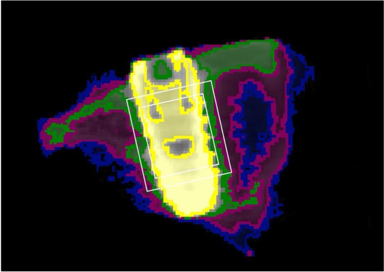
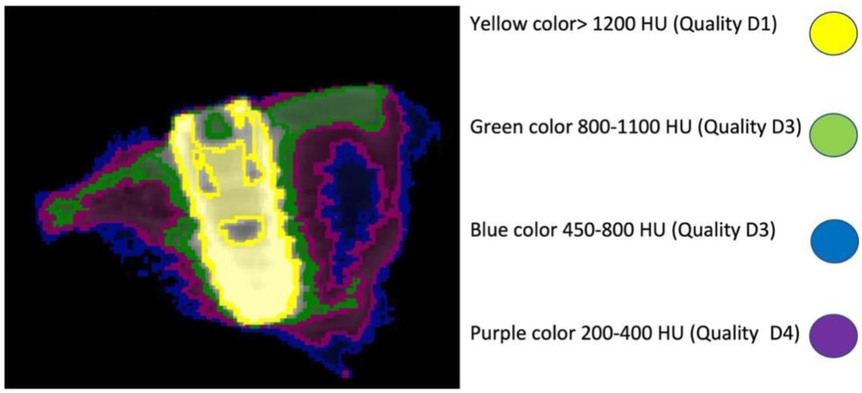
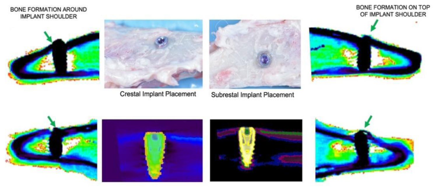
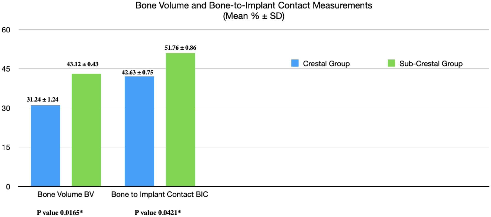
The primary purpose of this study was to determine the accuracy of micro-computed tomography (micro-CT) as a novel tool for the 3D analysis of bone density around dental implants in tibia rabbits. Six male New Zealand rabbits were used in our evaluation. One Copa SKY® (Bredent Medical GmbH & Co. K.G.) with a 3.5 mm diameter by 8.0 mm in length was placed within 12 tibia rabbits divided into two experimental groups: Group A (crestal placement) and Group B (sub-crestal placement). The animals were sacrificed at four weeks. Micro-CT evaluations showed a high amount of bone around all implants in the tibia rabbit bone. There was an increased formation of bone around the Copa SKY implants, mainly in the implants that were placed crestally. The most frequent density found in most implants was a medullary bone formation surrounding the implant; the density three (D3) was the most common type in all implants. The 3D model analysis revealed a mean bone volume (B.V.) of 31.24 ± 1.24% in crestal implants compared with the 43.12 ± 0.43% in sub-crestal implants. The mean actual contact implant to bone (B.I.C.) in the sub-crestal group was 51.76 ± 0.86%, compared to the 42.63 ± 0.75% in the crestal group. Compared to crestal implants, the Copa Sky implant placed sub-crestally allows for the formation of bone on top of the neck, thereby stimulating bone growth in tibia rabbits.
Citation: José Luis Calvo-Guirado, Marta Belén Cabo-Pastor, Félix de Carlos-Villafranca, Nuria García-Carrillo, Manuel Fernández-Domínguez, Francisco Martínez Martínez. Micro-CT evaluation of bone grow concept of an implant with microstructured backtaper crestally and sub-crestally placed. Preliminary study in New Zealand rabbits tibia at one month[J]. AIMS Bioengineering, 2023, 10(4): 406-420. doi: 10.3934/bioeng.2023024
The primary purpose of this study was to determine the accuracy of micro-computed tomography (micro-CT) as a novel tool for the 3D analysis of bone density around dental implants in tibia rabbits. Six male New Zealand rabbits were used in our evaluation. One Copa SKY® (Bredent Medical GmbH & Co. K.G.) with a 3.5 mm diameter by 8.0 mm in length was placed within 12 tibia rabbits divided into two experimental groups: Group A (crestal placement) and Group B (sub-crestal placement). The animals were sacrificed at four weeks. Micro-CT evaluations showed a high amount of bone around all implants in the tibia rabbit bone. There was an increased formation of bone around the Copa SKY implants, mainly in the implants that were placed crestally. The most frequent density found in most implants was a medullary bone formation surrounding the implant; the density three (D3) was the most common type in all implants. The 3D model analysis revealed a mean bone volume (B.V.) of 31.24 ± 1.24% in crestal implants compared with the 43.12 ± 0.43% in sub-crestal implants. The mean actual contact implant to bone (B.I.C.) in the sub-crestal group was 51.76 ± 0.86%, compared to the 42.63 ± 0.75% in the crestal group. Compared to crestal implants, the Copa Sky implant placed sub-crestally allows for the formation of bone on top of the neck, thereby stimulating bone growth in tibia rabbits.

| [1] |
Lehmann TM, Meinzer HP, Tolxdorff T (2004) Advances in biomedical image analysis. Methods Inf Med 43: 308-314. https://doi.org/10.1055/s-0038-1633873 
|
| [2] |
Handels H, Mersmann S, Palm C, et al. (2013) Viewpoints on medical image processing: from science to application. Curr Med Imaging 9: 79-88. https://doi.org/10.2174/1573405611309020002
|
| [3] |
Bouxsein ML, Boyd SK, Christiansen BA, et al. (2010) Guidelines for assessment of bone microstructure in rodents using micro–computed tomography. J Bone Miner Res 25: 1468-1486. https://doi.org/10.1002/jbmr.141
|
| [4] |
Höhne KH, Bomans M, Pommert A, et al. (1990) 3D visualization of tomographic volume data using the generalized voxel model. Vis Comput 6: 28-36. https://doi.org/10.1007/BF01902627
|
| [5] |
Beister M, Kolditz D, Kalender WA (2012) Iterative reconstruction methods in X-ray CT. Phys Med 28: 94-108. https://doi.org/10.1016/j.ejmp.2012.01.003
|
| [6] | Garland LH (1994) On the scientific evaluation of diagnostic procedures: Presidential address thirty-fourth annual meeting of the radiological society of North America. Radiology 19452: 309-328. https://doi.org/10.1148/52.3.309 |
| [7] |
Berlin L (2014) Radiologic errors, past, present, and future. Diagnosis 1: 79-84. https://doi.org/10.1515/dx-2013-0012
|
| [8] |
Bruno MA, Walker EA, Abujudeh HH (2015) Understanding and confronting our mistakes: The epidemiology of error in radiology and strategies for error reduction. Radiographic 35: 1668-1676. https://doi.org/10.1148/rg.2015150023
|
| [9] |
Waite S, Scott J, Gale B, et al. (2017) Interpretive error in radiology. Am J Roentgenol 208: 739-749. https://doi.org/10.2214/AJR.16.16963
|
| [10] |
Castellino RA (2005) Computer aided detection (CAD): an overview. Cancer Imaging 5: 17-19. https://doi.org/10.1102/1470-7330.2005.0018
|
| [11] |
Doi K (2007) Computer-aided diagnosis in medical imaging: historica review, current status and future potential. Comput Med Imaging Graph 31: 198-211. https://doi.org/10.1016/j.compmedimag.2007.02.002
|
| [12] |
Parrilla-Almansa A, García-Carrillo N, Ros-Tárraga P (2018) Demineralized bone matrix coating Si-Ca-P ceramic does not improve the osseointegration of the scaffold. Materials 11: 1580. https://doi.org/10.3390/ma11091580
|
| [13] |
Scarano A, Lorusso F, Orsini T, et al. (2019) Biomimetic surfaces coated with covalently immobilized collagen type I: An X-Ray photoelectron spectroscopy, atomic force microscopy, Micro-CT and histomorphometrical study in rabbits. Int J Mol Sci 20: 724. https://doi.org/10.3390/ijms20030724
|
| [14] |
Martinez IM, Velasquez PA, de Aza PN (2010) Synthesis and stability of tricalcium phosphate doped with dicalcium silicate in the system Ca3(PO4)2–Ca2SiO4. Mater Charact 61: 761-767. https://doi.org/10.1016/j.matchar.2010.04.010
|
| [15] |
Kim SY, Kim YK, Park YH, et al. (2017) Evaluation of the healing potential of demineralized dentin matrix fixed with recombinant human bone: morphogenetic protein-2 in bone grafts. Materials 10: 1049. https://doi.org/10.3390/ma10091049
|
| [16] |
Parrilla-Almansa A, González-Bermúdez CA, Sánchez-Sánchez S, et al. (2019) Intraosteal behavior of porous scaffolds: The mCT raw-data snalysis as a tool for better understanding. Symmetry 11: 532. https://doi.org/10.3390/sym11040532
|
| [17] | Trisi P, Lazzara R, Rao W, et al. (2002) Bone-implant contact and bone quality: Evaluation of expected and actual bone contact on machined and Osseotite implant surfaces. Int J Periodontics Restorative Dent 22: 535-545. |
| [18] | Rebaudi A, Laffi N, Benedicenti S, et al. (2011) Microcomputed tomographic analysis of bone reaction at insertion of orthodontic mini-implants in sheep. Int J Oral Maxillofac Implants 26: 1233-1240. |
| [19] |
Rueda AN, Ruiz-Trejo C, López-Pineda E, et al. (2021) Dosimetric evaluation in micro-CT studies used in preclinical molecular imaging. Appl Sci 11: 7930. https://doi.org/10.3390/app11177930
|
| [20] |
Calvo-Guirado JL, Ortiz-Ruiz AJ, Negri B, et al. (2010) Histological and histomorphometric evaluation of immediate implant placement on a dog model with a new implant surface treatment. Clin Oral Implants Res 21: 308-315. https://doi.org/10.1111/j.1600-0501.2009.01841.x
|
| [21] |
Sánchez F, Orero A, Soriano A, et al. (2013) ALBIRA: a small animal PET∕SPECT∕CT imaging system. Med Phys 40: 051906. https://doi.org/10.1118/1.4800798
|
| [22] |
Calvo-Guirado JL, García Carrillo Nuria, de Carlos-Villafranca Félix, et al. (2022) A micro-CT evaluation of bone density around two different types of surfaces on one-piece fixo implants with early loading-an experimental study in dogs at 3 months. AIMS Bioeng 9: 383-399. https://doi.org/10.3934/bioeng.2022028
|
| [23] |
Calvo-Guirado JL, Carlos-Villafranca Fd, Garcés-Villalá M, et al. (2022) X-ray micro-computed tomography characterization of autologous teeth particle used in postextraction sites for bone regeneration. An experimental study in dogs. Indian J Dent Sci 14: 58-67. https://doi.org/10.4103/ijds.ijds_138_21
|
| [24] |
Calvo‑Guirado JL, Carlos‑Villafranca FD, Garcés‑Villalá MA, et al. (2022) How much disinfected ground tooth do we need to fill an empty alveolus after extraction? Experimental in vitro study. Indian J Dent Sci 14: 171-177. https://doi.org/10.4103/ijds.ijds_24_22
|
| [25] |
Al Deeb M, Aldosari AAF, Anil S (2023) Osseointegration of tantalum trabecular metal in titanium dental implants: histological and micro-CT study. J Funct Biomater 14: 355. https://doi.org/10.3390/jfb14070355
|
| [26] | Anil S, Cuijpers VMJI, Preethanath RS, et al. (2013) Osseointegration of oral implants after delayed placement in rabbits: a microcomputed tomography and histomorphometric study. Int J Oral Max Impl 28: 1506-1511. https://doi.org/10.11607/jomi.3133 |
| [27] |
Pinotti FE, Aroni MAT, Oliveira GJPL, et al. (2023) Osseointegration of implants with superhydrophilic surfaces in rats with high serum levels of nicotine. Braz Dent J 34: 105-112. https://doi.org/10.1590/0103-6440202305096
|
| [28] |
Kunnekel AT, Dudani MT, Nair CK, et al. (2011) Comparison of delayed implant placement vs immediate implant placement using resonance frequency analysis: a pilot study on rabbits. J Oral Implantol 37: 543-548. https://doi.org/10.1563/AAID-JOI-D-10-00022.1
|
| [29] |
Bansal J, Kedige S, Bansal A, et al. (2012) A relaxed implant bed: Implants placed after two weeks of osteotomy with immediate loading: a one year clinical trial. J Oral Implantol 38: 155-164. https://doi.org/10.1563/AAID-JOI-D-10-00036
|
| [30] |
López-Valverde N, López-Valverde A, Cortés M P, et al. (2022) Bone quantification around chitosan-coated titanium dental implants: A preliminary study by micro-CT analysis in jaw of a canine model. Front Bioeng Biotechnol 10: 858786. https://doi.org/10.3389/fbioe.2022.858786
|
| [31] |
Berglundh T, Abrahamsson I, Lang NP, et al. (2003) De novo alveolar bone formation adjacent to endosseous implants. Clin Oral Implants Res 14: 251-262. https://doi.org/10.1034/j.1600-0501.2003.00972.x
|
| [32] |
Franchi M, Fini M, Martini D, et al. (2005) Biological fixation of endosseous implants. Micron 36: 665-671. https://doi.org/10.1016/j.micron.2005.05.010
|
| [33] |
Calvo-Guirado JL, Delgado-Peña J, Maté-Sánchez JE, et al. (2015) Novel hybrid drilling protocol: evaluation for the implant healing-thermal changes, crestal bone loss, and bone-to-implant contact. Clin Oral Implants Res 26: 753-760. https://doi.org/10.1111/clr.12341
|
| [34] |
Futami T, Fujii N, Ohnishi H, et al. (2000) Tissue response to titanium implants in the rat maxilla: Ultrastructural and histochemical observations of the bone-titanium interface. J Periodontol 71: 287-298. https://doi.org/10.1902/jop.2000.71.2.287
|
| [35] |
Castaneda S, Largo R, Calvo E, et al. (2006) Bone mineral measurements of subchondral and trabecular bone in healthy and osteoporotic rabbits. Skeletal Radiol 35: 34-41. https://doi.org/10.1007/s00256-005-0022-z
|
| [36] | Gilsanz V, Roe TF, Gibbens DT, et al. (1988) Effect of sex steroids on peak bone density of growing rabbits. Am J Physiol 255: E416-E421. https://doi.org/10.1152/ajpendo.1988.255.4.E416 |
| [37] |
Calvo-Guirado JL, Aguilar-Salvatierra A, Gomez-Moreno G, et al. (2014) Histological, radiological and histomorphometric evaluation of immediate vs. non-immediate loading of a zirconia implant with surface treatment in a dog model. Clin Oral Implants Res 25: 826-830. https://doi.org/10.1111/clr.12145
|
| [38] | Rodríguez-Ciurana X, Vela-Nebot X, Segala-Torres M, et al. (2009) The effect of interimplant distance on the height of the interimplant bone crest when using platform-switched implants. Int J Periodont Rest 29: 141-151. |
| [39] |
Romanos GE, Delgado-Ruiz RA, Nicolas-Silvente AI (2020) Volumetric changes in morse taper connections after implant placement in dense bone. In-vitro study. Materials 13: 2306. https://doi.org/10.3390/ma13102306
|
| [40] |
Delgado-Ruiz RA, Calvo-Guirado JL, Abboud M, et al. (2015) Connective tissue characteristics around healing abutments of different geometries: new methodological technique under circularly polarized light. Clin Implant Dent Relat Res 17: 667-680. https://doi.org/10.1111/cid.12161
|
| [41] |
Negri B, Calvo Guirado JL, Maté Sánchez de Val JE, et al. (2014) Peri-implant tissue reactions to immediate nonocclusal loaded implants with different collar design: an experimental study in dogs. Clin Oral Implants Res 25: 54-63. https://doi.org/10.1111/clr.12047
|
| [42] |
Calvo-Guirado JL, Boquete-Castro A, Negri B, et al. (2014) Crestal bone reactions to immediate implants placed at different levels in relation to crestal bone. A pilot study in Foxhound dogs. Clin Oral Implants Res 25: 344-351. https://doi.org/10.1111/clr.12110
|
| [43] |
Sotto-Maior BS, Lima Cde A, Senna PM, et al. (2014) Biomechanical evaluation of subcrestal dental implants with different bone anchorages. Braz Oral Res 28: 1-7. https://doi.org/10.1590/1807-3107BOR-2014.vol28.0023
|
| [44] |
Calvo-Guirado JL, López-López PJ, Mate Sanchez JE, et al. (2014) Crestal bone loss related to immediate implants in crestal and subcrestal position: a pilot study in dogs. Clin Oral Implants Res 25: 1286-1294. https://doi.org/10.1111/clr.12267
|
| [45] |
Calvo-Guirado JL, Delgado Ruiz RA, Ramírez-Fernández MP, et al. (2016) Histological and histomorphometric analyses of narrow implants, crestal and subcrestally placed in severe alveolar atrophy: a study in foxhound dogs. Clin Oral Implants Res 27: 497-504. https://doi.org/10.1111/clr.12569
|
| [46] |
Sánchez-Siles M, Muñoz-Cámara D, Salazar-Sánchez N, et al. (2018) Crestal bone loss around submerged and non-submerged implants during the osseointegration phase with different healing abutment designs: a randomized prospective clinical study. Clin Oral Implants Res 29: 808-812. https://doi.org/10.1111/clr.12981
|
| [47] |
de Siqueira RAC, Savaget Gonçalves Junior R, Dos Santos PGF, et al. (2020) Effect of different implant placement depths on crestal bone levels and soft tissue behavior: a 5-year randomized clinical trial. Clin Oral Implants Res 31: 282-293. https://doi.org/10.1111/clr.13569
|
| [48] |
de Siqueira RAC, Fontão FNGK, Sartori IAM, et al. (2017) Effect of different implant placement depths on crestal bone levels and soft tissue behavior: a randomized clinical trial. Clin Oral Implants Res 28: 1227-1233. https://doi.org/10.1111/clr.12946
|
| [49] |
Fernández-Domínguez M, Ortega-Asensio V, Fuentes Numancia E, et al. (2019) Can the macrogeometry of dental implants influence guided bone regeneration in buccal bone defects? Histomorphometric and biomechanical analysis in beagle dogs. J Clin Med 8: 618. https://doi.org/10.3390/jcm8050618
|
| [50] |
Yu YJ, Zhu WQ, Xu LN, et al. (2019) Osseointegration of titanium dental implant under fluoride exposure in rabbits: Micro-CT and histomorphometry study. Clin Oral Implants Res 30: 1038-1048. https://doi.org/10.1111/clr.13517
|
| [51] |
Scarano A, Orsini T, Di Carlo F, et al. (2021) Graphene-doped poly (methyl-methacrylate)(PMMA) implants: a micro-CT and histomorphometrical study in rabbits. Int J Mol Sci 22: 1441. https://doi.org/10.3390/ijms22031441
|
| [52] |
Negri B, Calvo-Guirado JL, Pardo Zamora G, et al. (2012) Peri-implant bone reactions to immediate implants placed at different levels in relation to crestal bone. Part I: a pilot study in dogs. Clin Oral Implants Res 23: 228-235. https://doi.org/10.1111/j.1600-0501.2011.02158.x
|
| [53] |
Putri A, Pramanik F, Azhari A (2023) Micro computed tomography and immunohistochemistry analysis of dental implant osseointegration in animal experimental model: a scoping review. Eur J Dent 17: 623-628. https://doi.org/10.1055/s-0042-1757468
|
| [54] |
Zhi Q, Zhang Y, Wei J, et al. (2023) Cell responses to calcium- and protein-conditioned titanium: an in vitro study. J Funct Biomater 14: 253. https://doi.org/10.3390/jfb14050253
|
| [55] |
Scarano A, Tari Rexhep S, Leo L, et al. (2023) Wettability of implant surfaces: Blood vs autologous platelet liquid (APL). J Mech Behav Biomed Mater 126: 104773. https://doi.org/10.1016/j.jmbbm.2021.104773
|
| [56] |
Silva IR, Barreto ATS, Seixas RS, et al. (2023) Novel strategy for surface modification of titanium implants towards the improvement of osseointegration property and antibiotic local delivery. Materials 16: 2755. https://doi.org/10.3390/ma16072755
|
| [57] |
Van Oossterwyck H, Duyck J, Vander Sloten J, et al. (2000) Use of microfocus computerized tomography as a new technique for characterizing bone tissue around oral implants. J Oral Implantol 26: 5-12. https://doi.org/10.1563/1548-1336
|
Figures(8) / Tables(2)

José Luis Calvo-Guirado, Marta Belén Cabo-Pastor, Félix de Carlos-Villafranca, Nuria García-Carrillo, Manuel Fernández-Domínguez, Francisco Martínez Martínez. Micro-CT evaluation of bone grow concept of an implant with microstructured backtaper crestally and sub-crestally placed. Preliminary study in New Zealand rabbits tibia at one month[J]. AIMS Bioengineering, 2023, 10(4): 406-420. doi: 10.3934/bioeng.2023024


 DownLoad: