Avena sterilis subsp. sterilis (sterile oat) is a troublesome grass weed of winter cereals both in its native range encompassing the Mediterranean up to South Asia, and in regions of America, Northern Europe and Australia where it is introduced. A better understanding of seedling emergence patterns of this weed in cereal fields can help control at early growth stages benefiting efficacy under a changing climate. With this aim, the objective of this research was to develop and validate a field emergence model for this weed based on cumulative air thermal time (CTT, ℃ day). Experiments for model setting and evaluation were carried out in experimental and commercial fields in southern Spain. Two alternative models, Gompertz and Weibull, were compared for their ability to represent emergence time course. The Weibull model provided the best fit to the data. Evaluation through independent experiments showed good model performance in predicting seedling emergence. According to the developed model, the onset of emergence takes place at 130 CTT, and 50% and 90% emergence is achieved at 448 and 632 CTT, respectively. Results indicate that this model could be useful for growers as a tool for decision-making in A. sterilis control.
Citation: Fernando Bastida, Kambiz Mootab Laleh, Jose L. Gonzalez-Andujar. Using air thermal time to predict the time course of seedling emergence of Avena sterilis subsp. sterilis (sterile oat) under Mediterranean climate[J]. AIMS Agriculture and Food, 2022, 7(2): 241-249. doi: 10.3934/agrfood.2022015
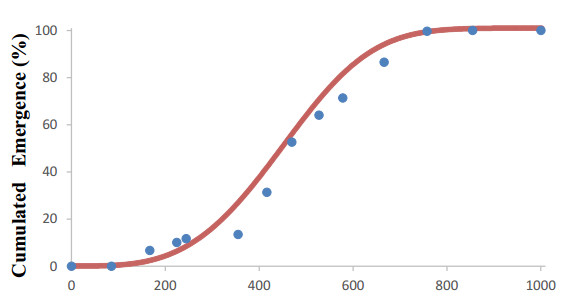
Avena sterilis subsp. sterilis (sterile oat) is a troublesome grass weed of winter cereals both in its native range encompassing the Mediterranean up to South Asia, and in regions of America, Northern Europe and Australia where it is introduced. A better understanding of seedling emergence patterns of this weed in cereal fields can help control at early growth stages benefiting efficacy under a changing climate. With this aim, the objective of this research was to develop and validate a field emergence model for this weed based on cumulative air thermal time (CTT, ℃ day). Experiments for model setting and evaluation were carried out in experimental and commercial fields in southern Spain. Two alternative models, Gompertz and Weibull, were compared for their ability to represent emergence time course. The Weibull model provided the best fit to the data. Evaluation through independent experiments showed good model performance in predicting seedling emergence. According to the developed model, the onset of emergence takes place at 130 CTT, and 50% and 90% emergence is achieved at 448 and 632 CTT, respectively. Results indicate that this model could be useful for growers as a tool for decision-making in A. sterilis control.

| [1] | IPNI (2021) International Plant Names Index. The Royal Botanic Gardens, Kew, Harvard University Herbaria & Libraries and Australian National Botanic Gardens. Available from: http://www.ipni.org. |
| [2] |
Barroso J, Alcantara C, Saavedra MM (2011) Competition between Avena sterilis ssp. sterilis and wheat in South Western Spain. Span J Agric Res 9: 862–872. https://doi.org/10.5424/sjar/20110903-403-10 doi: 10.5424/sjar/20110903-403-10

|
| [3] | Palma V, Saavedra MM, Garcia-Torres L (1990) Dinámica de poblaciones de Avena sterilis ssp sterilis L. en trigo (Triticum aestivum L.). Proceedings of the 1990 Spanish Weed Society Conference, Madrid, Spain, 285–289. |
| [4] |
Papapanagiotou AP, Damalas CA, Menexes GC, et al. (2020) Resistance levels and chemical control options of sterile oat (Avena sterilis L.) in Northern Greece. Int J Pest Manag 66: 106–115. https://doi.org/10.1080/09670874.2019.1569285 doi: 10.1080/09670874.2019.1569285
|
| [5] |
Armengot L, Jose-Maria L, Chamorro L, et al. (2017) Avena sterilis and Lolium rigidum infestations hamper the recovery of diverse arable weed communities. Weed Res 57: 278–286. https://doi.org/10.1111/wre.12254 doi: 10.1111/wre.12254
|
| [6] |
Pallavicini Y, Bastida F, Hernandez-Plaza E, et al. (2020) Local factors rather than the landscape context explain species richness and functional trait diversity and responses of plant assemblages of Mediterranean cereal field margins. Plants 9: 778. https://doi.org/10.3390/plants9060778 doi: 10.3390/plants9060778
|
| [7] | Heap I (2021) International survey of herbicide resistant weeds-weedscience.org. Available from: http://www.weedscience.org. |
| [8] |
Ngow Z, Chynoweth RJ, Gunnarsson M, et al. (2020) A herbicide resistance risk assessment for weeds in wheat and barley crops in New Zealand. PLoS ONE 15: e0234771. https://doi.org/10.1371/journal.pone.0234771 doi: 10.1371/journal.pone.0234771
|
| [9] |
Storkey J, Helps J, Hull R, et al. (2021) Defining integrated weed management: A novel conceptual framework for models. Agronomy 11: 747. https://doi.org/10.3390/agronomy11040747 doi: 10.3390/agronomy11040747
|
| [10] |
Calado JMG, Basch G, de Carvalho M (2009) Weed emergence as influenced by soil moisture and air temperature. J Pest Sci 82: 81–88. https://doi.org/10.1007/s10340-008-0225-x doi: 10.1007/s10340-008-0225-x
|
| [11] |
Tozzi E, Beckie H, Weiss R, et al. (2014) Seed germination response to temperature for of a range of international populations of Conyza canadensis. Weed Res 54: 178–185. https://doi.org/10.1111/wre.12065 doi: 10.1111/wre.12065
|
| [12] |
Grundy AC (2003) Predicting weed emergence: A review of approaches and future challenges. Weed Res 43: 1–11. https://doi.org/10.1046/j.1365-3180.2003.00317.x doi: 10.1046/j.1365-3180.2003.00317.x
|
| [13] |
Gonzalez-Andujar JL, Chantre GR, Morvillo C, et al. (2016) Predicting field weed emergence with empirical models and soft computing techniques. Weed Res 56: 415–423. https://doi.org/10.1111/wre.12223 doi: 10.1111/wre.12223
|
| [14] | Royo-Esnal A, Torra J, Chantre GR (2020) Weed Emergence Models. In: Chantre G, Gonzalez-Andujar JL (Eds.), Decision Support Systems for Weed Management, Springer, Cham. https://doi.org/10.1007/978-3-030-44402-0_5 |
| [15] |
Forcella F, Benech-Arnold R, Sánchez R, et al. (2000). Modelling seedling emergence. Field Crops Res 67: 123–139. https://doi.org/10.1016/S0378-4290(00)00088-5 doi: 10.1016/S0378-4290(00)00088-5
|
| [16] |
Grundy AC, Peters NCB, Rasmussen IA, et al. (2003) Emergence of Chenopodium album and Stellaria media of different origins under different climatic conditions. Weed Res 43: 163–176. https://doi.org/10.1046/j.1365-3180.2003.00330.x doi: 10.1046/j.1365-3180.2003.00330.x
|
| [17] |
Yousefi AR, Oveisi M, Gonzalez-Andujar JL (2014) Prediction of annual weed seedling emergence in garlic (Allium sativum L.) using soil thermal time. Sci Hortic 168: 189–192. https://doi.org/10.1016/j.scienta.2014.01.035 doi: 10.1016/j.scienta.2014.01.035
|
| [18] | Leguizamon ES, Fernandez-Quintanilla C, Barroso J, et al. (2005) Using thermal and hydrothermal time to model seedling emergence of Avena sterilis ssp. ludoviciana in Spain. https://doi.org/10.1111/j.1365-3180.2004.00444.xWeedRes45: 149–156. |
| [19] |
Sousa-Ortega C, Royo-Esnal A, Loureiro I, et al. (2021) Modelling emergence of sterile oat (Avena sterilis spp. ludoviciana) under semi-arid conditions. Weed Sci 69: 341–352. https://doi.org/10.1017/wsc.2021.10 doi: 10.1017/wsc.2021.10
|
| [20] |
Gonzalez-Andujar JL, Saavedra M (2003) Spatial distribution of annual grass weed populations in winter cereals. Crop Prot 22:629–633. https://doi.org/10.1016/S0261-2194(02)00247-8 doi: 10.1016/S0261-2194(02)00247-8
|
| [21] | Fernandez-Quintanilla C, Navarrete L, Torner C, et al. (1997) Avena sterilis L. en cultivos de cereales. In: Sans FX, Fernaandez-Quintanilla C (Eds.), Biología de las malas hierbas de España, Phytoma, Valencia, Spain, 77–89. |
| [22] | Romero-Zarco C (1987) Avena L. In: Valdes B, Talavera S, Fernandez-Galiano E, (Eds.), Flora vascular de Andalucía Occidental, Barcelona: Ketres Ed., 302–308. |
| [23] |
Castellanos-Frias E, Garcia De Leon D, Pujadas A, et al. (2014) Potential distribution of Avena sterilis L. in Europe under climate change. Annals Appl Biol 165: 53–61. https://doi.org/10.1111/aab.12117 doi: 10.1111/aab.12117
|
| [24] |
Leblanc ML, Cloutier DC, Leroux GD, et al. (1998) Facteurs impliqués dans la levée des mauvaises herbes au champ. Phytoprotection 79: 111–127. https://doi.org/10.7202/706140ar doi: 10.7202/706140ar
|
| [25] |
Fernandez-Quintanilla C, Gonzalez-Andujar JL, Appleby A (1990) Characterization of the germination and emergence response to temperature and soil moisture of Avena fatua and A. sterilis. Weed Res 30: 289–295. https://doi.org/10.1111/j.1365-3180.1990.tb01715.x doi: 10.1111/j.1365-3180.1990.tb01715.x
|
| [26] |
Nash JE, Sutcliffe JV (1970) River flow forecasting through conceptual model. Part 1-A discussion of principles. J Hydrology 10: 282–290. https://doi.org/10.1016/0022-1694(70)90255-6 doi: 10.1016/0022-1694(70)90255-6
|
| [27] |
Bastida F, Lezaun JA, Gonzalez-Andujar JL (2021) A predictive model for the time course of seedling emergence of Phalaris brachystachys (short-spiked canary grass) in wheat fields. Spanish J Agric Res 19: e10SC02. https://doi.org/10.5424/sjar/2021193-17876 doi: 10.5424/sjar/2021193-17876
|
| [28] |
Burnham KP, Anderson DR, Huyvaert KP (2011) AIC model selection and multimodel inference in behavioral ecology: some background, observations, and comparisons. Behav Ecology Sociobiology 65: 23–35. https://doi.org/10.1007/s00265-010-1029-6 doi: 10.1007/s00265-010-1029-6
|
| [29] |
Roman E, Murphy S, Swanton C (2000) Simulation of Chenopodium album seedling emergence. Weed Sci 48: 217–224. https://doi.org/10.1614/0043-1745(2000)048[0217:SOCASE]2.0.CO;2 doi: 10.1614/0043-1745(2000)048[0217:SOCASE]2.0.CO;2
|
| [30] | Gonzalez-Andujar JL (2020) Introduction to Decision Support Systems. In: Chantre G, Gonzalez-Andujar JL (Eds.), Decision Support Systems for Weed Management, Springer, Cham. |
| [31] |
Fernandez-Quintanilla C, Navarrete L, Andujar JLG et al. (1986) Seedling recruitment and age-specific survivorship and reproduction in populations of Avena sterilis ssp. Ludoviciana (Durieu) Nyman. J Appl Ecology 23: 945-955. https://doi.org/10.2307/2403946 doi: 10.2307/2403946
|
| [32] |
Picapietra G, Gonzalez-Andujar JL, Acciaresi HA (2021) Predicting junglerice (Echinochloa colona L.) emergence as a function of thermal time in the humid pampas of Argentina. Int J Pest Manag 67: 328–337. https://doi.org/10.1080/09670874.2020.1778811 doi: 10.1080/09670874.2020.1778811
|
| [33] |
Grundy A, Mead A (2000) Modeling weed emergence as a function of meteorological records. Weed Sci 48: 594–603. https://doi.org/10.1614/0043-1745(2000)048[0594:MWEAAF]2.0.CO;2 doi: 10.1614/0043-1745(2000)048[0594:MWEAAF]2.0.CO;2
|
| [34] |
Izquierdo J, Gonzalez-Andujar JL, Bastida F, et al. (2009) A thermal time model to predict corn poppy (Papaver rhoeas) emergence in cereal fields. Weed Sci 57: 660–664. https://doi.org/10.1614/WS-09-043.1 doi: 10.1614/WS-09-043.1
|
| [35] |
Egea-Cobrero V, Bradley K, Calha I, et al. (2020) Validation of predictive empirical weed emergence models of Abutilon theophrasti Medik. based on intercontinental data. Weed Res 60: 297–302. https://doi.org/10.1111/wre.12428 doi: 10.1111/wre.12428
|

Figures(2)

Fernando Bastida, Kambiz Mootab Laleh, Jose L. Gonzalez-Andujar. Using air thermal time to predict the time course of seedling emergence of Avena sterilis subsp. sterilis (sterile oat) under Mediterranean climate[J]. AIMS Agriculture and Food, 2022, 7(2): 241-249. doi: 10.3934/agrfood.2022015


 DownLoad: