Power sector plays a crucial role in the development of a country. Rise in population and industrial expansion in developing countries are reason to burdenize the central grid. Pakistan is a country in its developing stages. About 58% of its total energy generation is contributed by fossil fuel based conventional plants for which the fuel costs plenteous amount. In these circumstances it is indispensable to exploit naturally available renewable resources for electricity generation. This study proposes a hybrid hydro-kinetic/Photovoltaic/Biomass system integrated with grid to serve electricity in a residential area of district Kotli in AJK Pakistan. By evaluating available resources and total load demand data of residential consumers, a system design is modelled in HOMER to get techno-economic and optimal design analysis of the purposed system. Using several configurations and combinations of available energy generation systems and then by comparing their results, the most optimum system design is achieved in terms of initial cost, operating cost, cost per unit and net present cost of the system. To further refine the results, the effect of variations of different parameters like load demand, water flow speed and solar irradiance on system is investigated by performing sensitivity analysis on the system. Final results demonstrate that the purposed system is cost-effective and efficient to meet the load demand.
Citation: Muti Ur Rehman Tahir, Adil Amin, Ateeq Ahmed Baig, Sajjad Manzoor, Anwar ul Haq, Muhammad Awais Asgha, Wahab Ali Gulzar Khawaja. Design and optimization of grid Integrated hybrid on-site energy generation system for rural area in AJK-Pakistan using HOMER software[J]. AIMS Energy, 2021, 9(6): 1113-1135. doi: 10.3934/energy.2021051
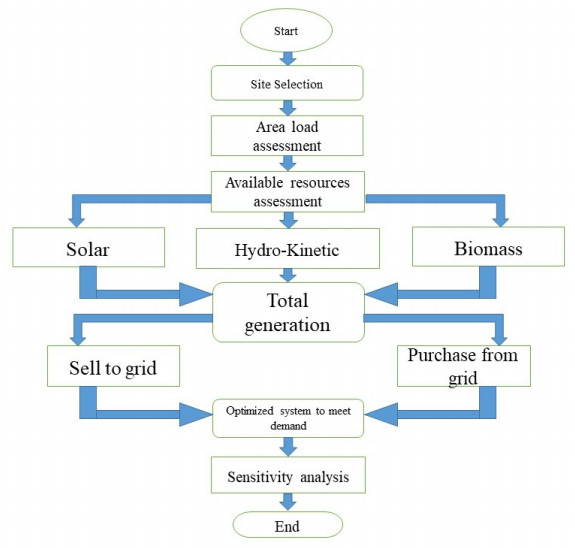
Power sector plays a crucial role in the development of a country. Rise in population and industrial expansion in developing countries are reason to burdenize the central grid. Pakistan is a country in its developing stages. About 58% of its total energy generation is contributed by fossil fuel based conventional plants for which the fuel costs plenteous amount. In these circumstances it is indispensable to exploit naturally available renewable resources for electricity generation. This study proposes a hybrid hydro-kinetic/Photovoltaic/Biomass system integrated with grid to serve electricity in a residential area of district Kotli in AJK Pakistan. By evaluating available resources and total load demand data of residential consumers, a system design is modelled in HOMER to get techno-economic and optimal design analysis of the purposed system. Using several configurations and combinations of available energy generation systems and then by comparing their results, the most optimum system design is achieved in terms of initial cost, operating cost, cost per unit and net present cost of the system. To further refine the results, the effect of variations of different parameters like load demand, water flow speed and solar irradiance on system is investigated by performing sensitivity analysis on the system. Final results demonstrate that the purposed system is cost-effective and efficient to meet the load demand.

| [1] | IRENA R E (2017) Accelerating the global energy transformation. International Renewable Energy Agency, Abu Dhabi. |
| [2] | HDIP P E Y (2009), Hydrocarbon Development Institute of Pakistan (HDIP). Islamabad. |
| [3] | Tribune T e. Thermal has largest share in Pakistan's energy mix. he express tribune 2020; Available from: https://tribune.com.pk/story/2240789/thermal-largest-share-pakistans-energy-mix. |
| [4] |
Farooq MK, Kumar S (2013) An assessment of renewable energy potential for electricity generation in Pakistan. Renewable Sustainable Energy Rev 20: 240–254. doi: 10.1016/j.rser.2012.09.042

|
| [5] | Government of pakistan finance division. Pakistan economic survey 2019–20. 2019–20; Available from: http://www.finance.gov.pk/survey_1920.html. |
| [6] | NEPRA State of industry report 2020. |
| [7] |
Qudrat-Ullah H (2015) Independent power (or pollution) producers? Electricity reforms and IPPs in Pakistan. Energy 83: 240–251. doi: 10.1016/j.energy.2015.02.018
|
| [8] |
Patt A, Lilliestam J (2018) The case against carbon prices. Joule 2: 2494–2498. doi: 10.1016/j.joule.2018.11.018
|
| [9] |
Mirza UK, Maroto-Valer MM, Ahmad N (2003) Status and outlook of solar energy use in Pakistan. Renewable Sustainable Energy Rev 7: 501–514. doi: 10.1016/j.rser.2003.06.002
|
| [10] | Ahmed MA, Ahmed F, Akhtar MW (2006) Assessment of wind power potential for coastal areas of Pakistan. Turkish J Phys 30: 127–135. |
| [11] |
Uddin W, Khan B, Shaukat N, et al. (2016) Biogas potential for electric power generation in Pakistan: A survey. Renewable Sustainable Energy Rev 54: 25–33. doi: 10.1016/j.rser.2015.09.083
|
| [12] | Government of pakistan finance division. Pakistan Economic Survey 2012–13. Available from: http://www.finance.gov.pk/survey_1213.html. |
| [13] |
Li J, Liu P, Li Z (2020) Optimal design and techno-economic analysis of a solar-wind-biomass off-grid hybrid power system for remote rural electrification: A case study of west China. Energy 208: 118387. doi: 10.1016/j.energy.2020.118387
|
| [14] |
Shahzad MK, Zahid A, Rashid T, et al. (2017) Techno-economic feasibility analysis of a solar-biomass off grid system for the electrification of remote rural areas in Pakistan using HOMER software. Renewable Energy 106: 264–273. doi: 10.1016/j.renene.2017.01.033
|
| [15] |
Ahmad J, Imran M, Khalid A, et al. (2018) Techno economic analysis of a wind-photovoltaic-biomass hybrid renewable energy system for rural electrification: A case study of Kallar Kahar. Energy 148: 208–234. doi: 10.1016/j.energy.2018.01.133
|
| [16] |
Chong WT, Naghavi MS, Poh SC, et al. (2011) Techno-economic analysis of a wind–solar hybrid renewable energy system with rainwater collection feature for urban high-rise application. Appl Energy 88: 4067–4077. doi: 10.1016/j.apenergy.2011.04.042
|
| [17] |
Krishan O, Suhag S (2019) Techno-economic analysis of a hybrid renewable energy system for an energy poor rural community. J Energy Storage 23: 305–319. doi: 10.1016/j.est.2019.04.002
|
| [18] | Kamran M, Asghar R, Mudassar M, et al. (2018) Designing and optimization of stand-alone hybrid renewable energy system for rural areas of Punjab, Pakistan. Int J Renewable Energy Res 8: 2385–2397. |
| [19] | Khan MU, Hassan M, Nawaz MH, et al. (2018) Techno-economic Analysis of PV/Wind/Biomass/Biogas Hybrid System for Remote Area Electrification of Southern Punjab (Multan), Pakistan using HOMER Pro. 2018 International Conference on Power Generation Systems and Renewable Energy Technologies (PGSRET), IEEE. |
| [20] |
Lata-García J, Jurado F, Fernández-Ramírez LM, et al. (2018) Optimal hydrokinetic turbine location and techno-economic analysis of a hybrid system based on photovoltaic/hydrokinetic/hydrogen/battery. Energy 159: 611–620. doi: 10.1016/j.energy.2018.06.183
|
| [21] |
Kalinci Y, Hepbasli A, Dincer I (2015) Techno-economic analysis of a stand-alone hybrid renewable energy system with hydrogen production and storage options. Int J Hydrogen Energy 40: 7652–7664. doi: 10.1016/j.ijhydene.2014.10.147
|
| [22] |
Jaszczur M, Hassan Q, Palej P, et al. (2020) Multi-Objective optimisation of a micro-grid hybrid power system for household application. Energy 202: 117738. doi: 10.1016/j.energy.2020.117738
|
| [23] |
Jaszczur M, Hassan Q (2020) An optimisation and sizing of photovoltaic system with supercapacitor for improving self-consumption. Appl Energy 279: 115776. doi: 10.1016/j.apenergy.2020.115776
|
| [24] |
Hassan Q (2021) Evaluation and optimization of off-grid and on-grid photovoltaic power system for typical household electrification. Renewable Energy 164: 375–390. doi: 10.1016/j.renene.2020.09.008
|
| [25] | Ali F, Jiang Y, Khan K (2017) Feasibility analysis of renewable based hybrid energy system for the remote community in Pakistan. 2017 IEEE International Conference on Industrial Engineering and Engineering Management (IEEM), IEEE. |
| [26] |
Ma T, Yang H, Lu L (2014) Development of a model to simulate the performance characteristics of crystalline silicon photovoltaic modules/strings/arrays. Sol Energy 100: 31–41. doi: 10.1016/j.solener.2013.12.003
|
| [27] | 2020, Available from: http://betapk.org/potential.html#:~:text=Each%20buffalo%2Fcow%20head%20can, of%20biogas%20(natural%20gas). |
| [28] |
Bhattacharya S, Thomas JM, Salam PA (1997) Greenhouse gas emissions and the mitigation potential of using animal wastes in Asia. Energy 22: 1079–1085. doi: 10.1016/S0360-5442(97)00039-X
|
| [29] | Plūme I, Dubrovskis V, Plūme B (2011) Specified evaluation of manure resources for production of biogas in planning region Latgale. Renewable Energy Energy Effic. |
| [30] |
Perera K, Rathnasiri PG, Senarath SAS, et al. (2005) Assessment of sustainable energy potential of non-plantation biomass resources in Sri Lanka. Biomass Bioenergy 29: 199–213. doi: 10.1016/j.biombioe.2005.03.008
|
| [31] |
Pazheri F, Othman M, Malik N (2014) A review on global renewable electricity scenario. Renewable Sustainable Energy Rev 31: 835–845. doi: 10.1016/j.rser.2013.12.020
|
| [32] |
Khan MJ, Bhuyan G, Iqbal MT, et al. (2009) Hydrokinetic energy conversion systems and assessment of horizontal and vertical axis turbines for river and tidal applications: A technology status review. Appl Energy 86: 1823–1835. doi: 10.1016/j.apenergy.2009.02.017
|
| [33] |
Gorlov A (1981) Hydrogen as an activating fuel for a tidal power plant. Int J Hydrogen Energy 6: 243–253. doi: 10.1016/0360-3199(81)90042-2
|
| [34] |
Lodhi M (1988) Power potential from ocean currents for hydrogen production. Int J Hydrogen Energy 13: 151–172. doi: 10.1016/0360-3199(88)90015-8
|
| [35] |
Yuce MI, Muratoglu A (2015) Hydrokinetic energy conversion systems: A technology status review. Renewable Sustainable Energy Rev 43: 72–82. doi: 10.1016/j.rser.2014.10.037
|
| [36] |
Koko SP, Kusakana K, Vermaak HJ (2015) Micro-hydrokinetic river system modelling and analysis as compared to wind system for remote rural electrification. Electr Power Syst Res 126: 38–44. doi: 10.1016/j.epsr.2015.04.018
|
| [37] |
Sood M, Singal SK (2019) Development of hydrokinetic energy technology: A review. Int J Energy Res 43: 5552–5571. doi: 10.1002/er.4529
|
| [38] |
Hu Z, X Du (2012) Reliability analysis for hydrokinetic turbine blades. Renewable Energy 48: 251–262. doi: 10.1016/j.renene.2012.05.002
|
| [39] |
Leopold LB (1953) Downstream change of velocity in rivers. Am J Sci 251: 606–624. doi: 10.2475/ajs.251.8.606
|
| [40] |
Arora VK, Boer GJ (1999) A variable velocity flow routing algorithm for GCMs. J Geophys Res: Atmos 104: 30965–30979. doi: 10.1029/1999JD900905
|
| [41] | Leopold LB, Maddock T (1953) The Hydraulic Geometry of Stream Channels and Some Physiographic Implications. |
| [42] |
Allen PM, Arnold JC, Byars BW (1994) Downstream channel geometry for use in planning‐level models. J Am Water Resour Assoc 30: 663–671. doi: 10.1111/j.1752-1688.1994.tb03321.x
|
| [43] | Mira Power Limited (MPL) I (2014) Environmental and Social Impact Assessment of Gulpur Hydropower Project, HBP Ref.: D4V01GHP. |
| [44] | Pakistan H B (2014), Cumulative Impact Assessment Gulpur Hydropower Project, HBP Ref.: R4R03GHP. |
| [45] | Anurag Kumar A p. (cited 2020 Cost Assessment of Hydrokinetic Power Generation. 2017); Available from: https://www.ijarse.com/images/fullpdf/1514970772_TE01-036.pdf. |
| [46] |
Miller VB, Ramde EW, Gradoville RT, et al. (2011) Hydrokinetic power for energy access in rural Ghana. Renewable Energy 36: 671–675. doi: 10.1016/j.renene.2010.08.014
|
| [47] | Johnson JB, Pride DJ (2010) River, tidal, and ocean current hydrokinetic energy technologies: status and future opportunities in Alaska. Prepared Alaska Center Energy Power. |
| [48] |
Rouhani M, Kish GJ (2019) Multiport DC–DC–AC modular multilevel converters for hybrid AC/DC power systems. IEEE Trans Power Delivery 35: 408–419. doi: 10.1109/TPWRD.2019.2927324
|
| [49] | Garmabdari R, Moghimi M, Yang F, et al. (2018) Energy storage sizing and optimal operation analysis of a grid-connected microgrid. International Conference on Sustainability in Energy and Buildings. |
| [50] |
Carpinelli G, Fazio AR, Khormali S, et al. (2014) Optimal sizing of battery storage systems for industrial applications when uncertainties exist. Energies 7: 130–149. doi: 10.3390/en7010130
|
| [51] |
Chen SX, Gooi HB, Wang M (2011) Sizing of energy storage for microgrids. IEEE Trans Smart Grid 3: 142–151. doi: 10.1109/TSG.2011.2160745
|


Figures(10) / Tables(9)

Muti Ur Rehman Tahir, Adil Amin, Ateeq Ahmed Baig, Sajjad Manzoor, Anwar ul Haq, Muhammad Awais Asgha, Wahab Ali Gulzar Khawaja. Design and optimization of grid Integrated hybrid on-site energy generation system for rural area in AJK-Pakistan using HOMER software[J]. AIMS Energy, 2021, 9(6): 1113-1135. doi: 10.3934/energy.2021051


 DownLoad: