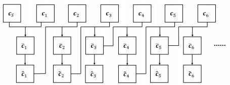
Figure 1.
The diagram of Step 5.


Citation: Zhilan Feng, Robert Swihart, Yingfei Yi, Huaiping Zhu. Coexistence in a metapopulation model with explicit local dynamics[J]. Mathematical Biosciences and Engineering, 2004, 1(1): 131-145. doi: 10.3934/mbe.2004.1.131
| [1] | Santosh Kumar Henge, Gitanjali Jayaraman, M Sreedevi, R Rajakumar, Mamoon Rashid, Sultan S. Alshamrani, Mrim M. Alnfiai, Ahmed Saeed AlGhamdi . Secure keys data distribution based user-storage-transit server authentication process model using mathematical post-quantum cryptography methodology. Networks and Heterogeneous Media, 2023, 18(3): 1313-1334. doi: 10.3934/nhm.2023057 |
| [2] | Rong Huang, Zhifeng Weng . A numerical method based on barycentric interpolation collocation for nonlinear convection-diffusion optimal control problems. Networks and Heterogeneous Media, 2023, 18(2): 562-580. doi: 10.3934/nhm.2023024 |
| [3] | Catherine Choquet, Ali Sili . Homogenization of a model of displacement with unbounded viscosity. Networks and Heterogeneous Media, 2009, 4(4): 649-666. doi: 10.3934/nhm.2009.4.649 |
| [4] | Edward S. Canepa, Alexandre M. Bayen, Christian G. Claudel . Spoofing cyber attack detection in probe-based traffic monitoring systems using mixed integer linear programming. Networks and Heterogeneous Media, 2013, 8(3): 783-802. doi: 10.3934/nhm.2013.8.783 |
| [5] | A. Marigo . Robustness of square networks. Networks and Heterogeneous Media, 2009, 4(3): 537-575. doi: 10.3934/nhm.2009.4.537 |
| [6] | Javier A. Almonacid, Gabriel N. Gatica, Ricardo Oyarzúa, Ricardo Ruiz-Baier . A new mixed finite element method for the n-dimensional Boussinesq problem with temperature-dependent viscosity. Networks and Heterogeneous Media, 2020, 15(2): 215-245. doi: 10.3934/nhm.2020010 |
| [7] | Tasnim Fatima, Ekeoma Ijioma, Toshiyuki Ogawa, Adrian Muntean . Homogenization and dimension reduction of filtration combustion in heterogeneous thin layers. Networks and Heterogeneous Media, 2014, 9(4): 709-737. doi: 10.3934/nhm.2014.9.709 |
| [8] | Mohamed Belhadj, Eric Cancès, Jean-Frédéric Gerbeau, Andro Mikelić . Homogenization approach to filtration through a fibrous medium. Networks and Heterogeneous Media, 2007, 2(3): 529-550. doi: 10.3934/nhm.2007.2.529 |
| [9] | Michael Herty, Lorenzo Pareschi, Giuseppe Visconti . Mean field models for large data–clustering problems. Networks and Heterogeneous Media, 2020, 15(3): 463-487. doi: 10.3934/nhm.2020027 |
| [10] | Jinhu Zhao . Natural convection flow and heat transfer of generalized Maxwell fluid with distributed order time fractional derivatives embedded in the porous medium. Networks and Heterogeneous Media, 2024, 19(2): 753-770. doi: 10.3934/nhm.2024034 |
The development of information technology leads to information security issues that have become a serious problem, so it is particularly important to develop the encryption technology. For example, traditional symmetric encryption has DES and AES encryption [1] etc., asymmetric encryption has RSA encryption [1] etc. Due to the large amount of data for image, the traditional encryption technology for image encryption effect is not prominent. Therefore, many encryption algorithms are proposed and improved, chaotic encryption system is the most widely used encryption method in recent years [2,3], such as the improved Henon map [4], 3D logistic-sine cascade map [5] and improved sine map [6]. In [7], a new chaotic system called delayed feedback dynamic mixed linear-nonlinear coupled mapping lattices (DFDMLNCML) is proposed, in [8], an image encryption algorithm based on a hidden attractor chaos system and Knuth-Durstenfeld algorithm is proposed, in [9], a chaos encryption algorithm combining Cyclic Redundancy Check (CRC) and nine palace map is proposed and in [10], a chaotic image encryption algorithm combined with frequency-domain DNA encoding is proposed. The authors of [11] applied speech recognition technology to chaotic cryptosystems. An image encryption algorithm based on dynamic row scrambling and Zigzag transformation is proposed in [12], the authors of [13] proposed a new chaotic pseudo-random number generator (CPRNG). A colour image encryption model based on two nearby orbits of chaotic systems is presented in [14]. At present, chaotic systems have also been widely used in various practical problems, such as medical images [15,16,17,18], secure wireless communication [19], IoT applications [20,21] and so on. In addition, many other encryption algorithms have been proposed in recent years, such as the image encryption algorithm based on self-adaptive diffusion and combined global scrambling [22], the image encryption algorithm based on 2-dimensional compressive sensing [23], the fast image encryption algorithm based on parallel computing system [24]. With the continuous development of encryption technology, new encryption algorithms are emerging. Therefore, the evaluation of encryption algorithms is more stringent, and some evaluation indexes are used to test the security and randomness of images, such as Statistical Test NIST SP 800-22 [25], Test U01 [26] and the 0–1 test [27] etc. Encryption technology is still in continuous development. Due to the emergence of various means of attack, the new encryption algorithm must and deserves to be proposed.
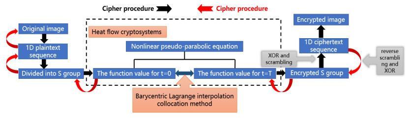
Different from traditional encryption technique, the heat flow cryptosystem is a new method that combines the cryptographic method with the partial differential equation [28], the core of the cryptosystem is a class of partial differential equation. The encryption and decryption process is realized by solving the equation to get the state function values at two moments, thus it is usually necessary to seek efficient and stable numerical methods to solve such equations. For the research of heat flow cryptosystem, many scholars have proposed the reliable numerical methods to solve the models, such as reproducing kernel method [29], pseudo-spectral method [30], finite element method [31], mixed volume element method [32], difference method [33] and so on. In addition, the model of heat flow cryptosystem is also applied to practical problems, such as image encryption [34], text and continuous signals encryption. In this paper, the barycentric Lagrange interpolation collocation method is adopted for heat flow cryptosystem. Barycentric interpolation collocation method is a meshless numerical method with high computation precision and efficiency [35], thus the numerical method has been widely used [36].
The main work of this paper is to propose an image encryption algorithm with high security, and then we use several common indicators to objectively evaluate the encryption algorithm. Block encryption is adopted and each group contains two diffusions and one scrambling process. The first diffusion changes the pixel value of the image through the nonlinear pseudo-parabolic equation. Further, each group is recombined into a matrix, matrix elements represent the pixel values after diffusion. The second diffusion performs bitwise XOR on each group and its previous group and we scramble the matrix, then each group performs the same operation. The encryption algorithm is sensitive to the pixel value of the first group. If a pixel value in the first group is changed, it will affect the diffusion effect of the subsequent groups. Therefore, the algorithm has strong key sensitivity and plaintext sensitivity. Compared with the common chaotic encryption system, the advantage of the heat flow cryptosystem is that the key space is so large, the key functions p(x,y) and q(x,y) can be any continuous function in the domain, so the selected p(x,y) and q(x,y) are infinite. Heat flow cryptosystem can effectively resist exhaustive attack by relying on this ability.
The structure of this article is organized as follows: in Section 2, the heat flow cryptosystem based on a class of (1+1)-dimensional and (2+1)-dimensional nonlinear pseudo-parabolic equations are given, the barycentric Lagrange interpolation to solve the nonlinear pseudo-parabolic equations is introduced. In Section 3, the image encryption algorithm based on this heat flow cryptosystem is designed, the flow diagram is also given. In Section 4, the decryption algorithm and flow diagram is given. In Section 5, several examples are given to support the proposed encryption algorithm.
In this section, the model of heat flow cryptosystem based on a (1+1)-dimensional nonlinear pseudo-parabolic equation is given [31]
| {(p(x)uxt)x+(p(x)ux)x−(q(x)+1)ut−q(x)u=f(x,t,r)+20xu2,u(x,0)=f0(x),u(0,t)=0,u(1,t)=0 | (2.1) |
and the model of heat flow cryptosystem based on (2+1)-dimensional nonlinear pseudo-parabolic equation is given [32]
| {∇⋅(p(x,y)∇ut)+∇⋅(p(x,y)∇u)−(q(x,y)−1)ut−q(x,y)u=f(x,y,t,r)+20xyu2,u(x,y,0)=f0(x,y),u(0,y,t)=0,u(1,y,t)=0,u(x,0,t)=0,u(x,1,t)=0, | (2.2) |
where (x,t)∈[0,1]×[0,T] for (1+1)-dimensional nonlinear pseudo-parabolic equation (2.1) and (x,y)∈Ω=[0,1]×[0,1], t∈[0,T] for (2+1)-dimensional nonlinear pseudo-parabolic equation Eq (2.2), T is the final time. p(x), q(x) in (2.1) and p(x,y), q(x,y) in Eq (2.2) are given functions, ∇ is Nabla operator and (∇⋅) is divergence operator. The r in formula (2.1) and (2.2) is a constant.
Let
| {S1[u]=(p(x)uxt)x+(p(x)ux)x−(q(x)+1)ut−q(x)u,S2[u]=∇⋅(p(x,y)∇ut)+∇⋅(p(x,y)∇u)−(q(x,y)−1)ut−q(x,y)u. |
We take the function values at t=0 (i.e., f0(x) and f0(x,y)) as plaintext and take u(x,T)=g0(x), u(x,y,T)=g0(x,y) as ciphertext, then the (1+1)-dimensional encryption model and decryption model can be expressed as
| {S1[u]=f(x,t,r)+20xu2,u(x,0)=f0(x),u(0,t)=0,u(1,t)=0,{S1[u]=f(x,t,r)+20xu2,u(x,T)=g0(x),u(0,t)=0,u(1,t)=0, | (2.3) |
(2+1)-dimensional encryption model and decryption model can be expressed as
| {S2[u]=f(x,y,t,r)+20xyu2,u(x,y,0)=f0(x,y),u(0,y,t)=0,u(1,y,t)=0,u(x,0,t)=0,u(x,1,t)=0,{S2[u]=f(x,y,t,r)+20xyu2,u(x,y,T)=g0(x,y),u(0,y,t)=0,u(1,y,t)=0,u(x,0,t)=0,u(x,1,t)=0. | (2.4) |
The p(x),q(x),p(x,y),q(x,y),f(x,t,r),f(x,y,t,r) and final time T are cryptographic key. The plaintext and ciphertext corresponding to the solution of u at two different times t=0 and t=T.
The (2+1)-dimensional nonlinear pseudo-parabolic equation (2.2) is taken as an example to construct the iterative scheme. We can obtain the simplified equation (2.2)
| (px+py)(uxt+uyt+ux+uy)+p(uxxt+uyyt+uxx+uyy)−(q+1)ut−qu=f(x,y,t,r)+20xyu2. | (2.5) |
Substituting the iterative initial value u0 into the nonlinear term of 20xyu2, the linearized equation can be obtained as
| (px+py)(uxt+uyt+ux+uy)+p(uxxt+uyyt+uxx+uyy)−(q+1)ut−qu=f(x,y,t,r)+20xyu20. | (2.6) |
The iterative scheme can be constructed by u→u(h), u0→u(h−1)
| (px+py)(u(h)xt+u(h)yt+u(h)x+u(h)y)+p(u(h)xxt+u(h)yyt+u(h)xx+u(h)yy)−(q+1)u(h)t−qu(h)=f(x,y,t,r)+20xy(u(h−1))2. | (2.7) |
Consider u(x,y,t)∈Ω=[a,b]×[c,d], the spatial region Ω is discretized into
| {Ωij=(xi,yj),i=1,2,⋯,m;j=1,2,⋯,n} |
and time region [0,T] is discretized into {tk,k=1,2,⋯,l}, Then we have tensor interpolation nodes
| {(xi,yj,tk),i=1,2,⋯,m;j=1,2,⋯,n;k=1,2,⋯,l} | (2.8) |
in the computational domain Ω×[0,T]. Defining uijk=u(xi,yj,tk), then the barycentric Lagrange interpolation polynomial of u(x,y,t) can be expressed as
| u(x,y,t)=m∑i=1n∑j=1l∑k=1Li(x)Mj(y)Tk(t)uijk, | (2.9) |
where Li(x), Mj(y), Tk(t) are the basic function, the corresponding expressions are
| {Li(x)=ωix−xim∑i=1ωix−xi,ωi=1m∏k=1,k≠i(xi−xk),{Mj(y)=νjy−yjn∑j=1νjy−yj,νj=1n∏k=1,k≠j(yj−yk),{Tk(t)=λkt−tkl∑k=1λkt−tk,λk=1l∏i=1,i≠k(tk−ti). |
Adopting Eq (2.9) to approximate the unknown function u in Eq (2.7) and make it hold at the interpolation node (2.8), then the iterative scheme (2.7) can be written in the matrix form (Ref. [37])
| Hu(h)=f+20xy(u(h−1))2, | (2.10) |
where
| H=(Px+Py)[(L(100)⊗In⊗L(001))+(Im⊗L(010)⊗L(001))+(L(100)⊗In⊗Il)+(Im⊗L(010)⊗Il)]+P[(L(200)⊗In⊗L(001))+(Im⊗L(020)⊗L(001))+(L(200)⊗In⊗Il)+(Im⊗L(020)⊗Il)]−(Q+Im⊗In⊗Il)(Im⊗In⊗L(001))−Q(Im⊗In⊗Il), |
| Px=diag(px)⊗Il,px=[px(x1,y1),px(x1,y2),⋯px(x1,yn),⋯,⋯,px(xm,y1),px(xm,y2),⋯px(xm,yn)]T, |
| Py=diag(py)⊗Il,py=[py(x1,y1),py(x1,y2),⋯py(x1,yn),⋯,⋯,py(xm,y1),py(xm,y2),⋯py(xm,yn)]T, |
| P=diag(p)⊗Il,p=[p(x1,y1),p(x1,y2),⋯p(x1,yn),⋯,⋯,p(xm,y1),p(xm,y2),⋯p(xm,yn)]T, |
| Q=diag(q)⊗Il,q=[q(x1,y1),q(x1,y2),⋯q(x1,yn),⋯,⋯,q(xm,y1),q(xm,y2),⋯q(xm,yn)]T, |
| f=[f111,f112,⋯,f11l,f121,f122,⋯,f12n,⋯,⋯,fmn1,fmn2,⋯,fmnl]T,fijk=f(xi,yj,tk), |
| u(h)=[u(h)111,u(h)112,⋯,u(h)11l,u(h)121,u(h)122,⋯,u(h)12l,⋯,⋯,u(h)mn1,u(h)mn2,⋯,u(h)mnl]T,u(h)ijk=u(h)(xi,yj,tk), |
| u(h−1)=[u(h−1)111,u(h−1)112,⋯,u(h−1)11l,u(h−1)121,u(h−1)122,⋯,u(h−1)12l,⋯,⋯,u(h−1)mn1,u(h−1)mn2,⋯,u(h−1)mnl]T, |
| u(h−1)ijk=u(h−1)(xi,yj,tk), |
where ⨂ is kronecker product, Im, In, Il are unit matrices with m-order, n-order, l-order, respectively. L(100) and L(200) are the 1-order and 2-order differential matrices with x. L(010) and L(020) are 1-order and 2-order differential matrices with y. L(001) is the 1-order differential matrices with t. The elements in differential matrix and the handling of initial-boundary condition are given in Ref.[37].
Let h=1, the matrix equation (2.10) begins iteration. The iterated precision E is given, when
| ||u(h)−u(h−1)||2=√(u(h)111−u(h−1)111)2+(u(h)112−u(h−1)112)2+⋯+(u(h)11l−u(h−1)11l)2+(u(h)121−u(h−1)121)2+(u(h)122−u(h−1)122)2+⋯+(u(h)12l−u(h−1)12l)2+⋯+⋯+(u(h)mn1−u(h−1)mn1)2+(u(h)mn2−u(h−1)mn2)2+⋯+(u(h)mnl−u(h−1)mnl)2≤E, | (2.11) |
iteration stop, we denote h=hend for the last iteration, the numerical solutions u(hend)ijk=u(hend)(xi,yj,tk),i=1,2,⋯,m;j=1,2,⋯,n;k=1,2,⋯,l can be obtained. When the k=1, the
| u(hend)t=0=[u(hend)111,u(hend)121,⋯,u(hend)1n1,u(hend)211,u(hend)221,⋯,u(hend)2n1,⋯,⋯,u(hend)m11,u(hend)m21,⋯,u(hend)mn1]T | (2.12) |
is the numerical solutions at t=0.
When the k=l, the
| u(hend)t=T=[u(hend)11l,u(hend)12l,⋯,u(hend)1nl,u(hend)21l,u(hend)22l,⋯,u(hend)2nl,⋯,⋯,u(hend)m1l,u(hend)m2l,⋯,u(hend)mnl]T | (2.13) |
is the numerical solutions at t=T.
In this section, an image encryption algorithm based on the above analysis is proposed.
Step 1 Consider an image A of size M×N (Height is M and Width is N), we expand pixels in column order to get a set of 1-dimensional sequences
| A={a11,a21,⋯,aM1,a12,a22,⋯,aM2,⋯,⋯,a1N,a2N,⋯,aMN}, |
where aij(i=1,2,⋯,M;j=1,2,⋯,N) is the pixel value of row i, column j in the image.
Step 2 Spliting A in order, 16 pixels as a group, we can obtain B={b1,b2,⋯,bS}, where bs(s=1,2,⋯,S) denote the group s. If the number of pixels in the last group bS is less than 16, we fill it with 0 pixels.
Step 3 Each group bs(s=1,2,⋯,S) is normalized, according to the distribution of pixels, the following three cases will be considered:
● If all pixel values are 0 in this group, we adopt the median 0.5 of [0,1] as the result of pixel normalization.
● If the pixel values are all equal and not 0 in this group, we use the weight of the pixel value in [0,255] as the normalized result. For example, if the pixel values in this group are all 241, then the normalized results are all 241/255=0.9451.
● If the pixel values are not all equal in this group, we use the formula
| b′sk=bsk−bsminbsmax−bsmin | (3.1) |
where bsk(s=1,2,⋯,S;k=1,2,⋯,16) denote the k-th pixel value in the group s, bsmax and bsmin denote the maximum and minimum pixel value in the group s, respectively, b′sk is the normalized result.
Then B′={b′1,b′2,⋯,b′S} can be obtained. Taking b′s as the initial condition f0 in model (2.3) or (2.4). The barycentric Lagrange interpolation collocation method introduced in Section 2 is adopted to solve the nonlinear pseudo-parabolic equation in model (2.3) or (2.4), then we can obtain the g0 in (2.3) or (2.4), we denote it by gs.
In the process, r∈[rmin,rmax] is a key parameter, where rmax is a given value and rmin is obtained by the original image
| {A(i)=A(i,1)⊕A(i,2)⊕⋯⊕A(i,N);i=1,2,⋯,M,E=A(1)⊕A(2)⊕⋯⊕A(M),rmin=25+mod(E,5), |
where ⊕ denote XOR, A(i,j)(i=1,2,⋯,M;j=1,2,⋯,N) denote the pixel of position (i,j) in original image, the mod() is the modular function. Each group b′s corresponds to an r. The growth step of r denote rh, the r for b′s is
| rs=rmin+(s−1)rh,s=1,2,⋯,S, |
in addition, a constraint condition is given: when r≥rmax, r start again from rmin according to the same rule. The value of r in the last group b′S is recorded as rend. We can get the {g1,g2,⋯,gS} and gs is normalized by use formula (3.1) to get g′s, then we have C={c1,c2,⋯,cS} by cs=g′s×255.
Step 4 For the cs∈C in Step 3, we combine them in column order into a matrix of size 4×4, we denote it into cs as follows
| cs=(cs(1)cs(5)cs(9)cs(13)cs(2)cs(6)cs(10)cs(14)cs(3)cs(7)cs(11)cs(15)cs(4)cs(8)cs(12)cs(16)),s=1,2,⋯,S, |
where cs(k)(k=1,2,⋯,16) denote the k-th pixel value in cs. The matrix sequence D formed by ds is denoted as C={c1,c2,⋯,cS}.
Step 5 For the c1∈C in Step 4,
| ¯c1=c1⊕cS=(c1(1)c1(5)c1(9)c1(13)c1(2)c1(6)c1(10)c1(14)c1(3)c1(7)c1(11)c1(15)c1(4)c1(8)c1(12)c1(16))⊕(cS(1)cS(5)cS(9)cS(13)cS(2)cS(6)cS(10)cS(14)cS(3)cS(7)cS(11)cS(15)cS(4)cS(8)cS(12)cS(16))=(¯c1(1)¯c1(5)¯c1(9)¯c1(13)¯c1(2)¯c1(6)¯c1(10)¯c1(14)¯c1(3)¯c1(7)¯c1(11)¯c1(15)¯c1(4)¯c1(8)¯c1(12)¯c1(16)), |
then we scramble ¯c1 according to the rule: the row i moves one position to the left and the column i moves one position up, where i=1,2,⋯,4, we have the scrambled matrix ˆc1
| ˆc1=(¯c1(2)¯c1(10)¯c1(14)¯c1(3)¯c1(6)¯c1(7)¯c1(15)¯c1(4)¯c1(8)¯c1(11)¯c1(12)¯c1(5)¯c1(9)¯c1(13)¯c1(16)¯c1(1)), |
¯c2 can be obtained by
| ¯c2=c2⊕ˆc1=(c2(1)c2(5)c2(9)c2(13)c2(2)c2(6)c2(10)c2(14)c2(3)c2(7)c2(11)c2(15)c2(4)c2(8)c2(12)c2(16))⊕(¯c1(2)¯c1(10)¯c1(14)¯c1(3)¯c1(6)¯c1(7)¯c1(15)¯c1(4)¯c1(8)¯c1(11)¯c1(12)¯c1(5)¯c1(9)¯c1(13)¯c1(16)¯c1(1))=(¯c2(1)¯c2(5)¯c2(9)¯c2(13)¯c2(2)¯c2(6)¯c2(10)¯c2(14)¯c2(3)¯c2(7)¯c2(11)¯c2(15)¯c2(4)¯c2(8)¯c2(12)¯c2(16)), |
we scramble ¯c2 according to the rule: the row j moves one position to the right and the column j moves one position down, where j=1,2,⋯,4, we have the scrambled matrix ˜c2
| ˜c2=(¯c2(4)¯c2(8)¯c2(12)¯c2(13)¯c2(14)¯c2(1)¯c2(5)¯c2(9)¯c2(15)¯c2(2)¯c2(6)¯c2(10)¯c2(16)¯c2(3)¯c2(7)¯c2(11)), |
Starting from c3,
| {¯cs=cs⊕˜cs−1,¯cs→ˆcsmod(s,2)≠0,s≥3¯cs=cs⊕ˆcs−1,¯cs→˜cs,mod(s,2)=0,s≥3 |
then the C={ˆc1,˜c2,ˆc3,˜c4,⋯} can be obtained. The diagram for Step 5 is shown in Figure 1.
Step 6 For the each matrix of C in Step 5, we expand it in column order, then a long 1-dimensional sequence can be obtained. Extracting the first MN elements and combine it into a matrix of size M×N in column order, then we can get the encrypted image.
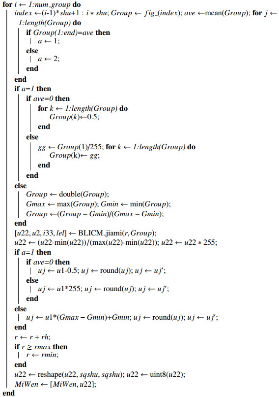
In Algorithm 1, we give the pseudo-code of Image preprocessing process corresponding to the Step 1 to Step 2. The Algorithm 2 shows the process of heat flow cryptosystem encryption in Step 3.
| Algorithm 1: Image preprocessing process |
Input: Image
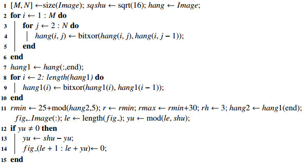
|
| Algorithm 2: Heat flow cryptosystem encryption |
num_group← length(fig_)/shu; MiWen←[];
|
In heat flow cryptosystem, the function value at final time can be obtained by taking the plaintext as the initial condition. The reverse process is to solve the function value at initial time by taking the final time function value as the initial condition. In addition, each step of encryption algorithm is reversible, so the decryption algorithm is the inverse process of encryption algorithm. The specific decryption algorithm process as follows.
Step 1 For the 1-dimensional sequence C in encryption algorithm Step 6, supposing the length of C is lC, recombining the C in column order into a matrix of size 4×(lC/4).
Step 2 Spliting the matrix C, one matrix of size 4×4 as a group, then the C={ˆc1,˜c2,ˆc3,˜c4,⋯} in encryption algorithm Step 5 can be obtained. Starting from the last group,
| {ˆcs→¯cs,cs=¯cs⊕˜cs−1,mod(s,2)≠0,s≠1,˜cs→¯cs,cs=¯cs⊕ˆcs−1,mod(s,2)=0,ˆc1→¯c1,c1=¯c1⊕cS,s=1, |
where the rule of ˆcs→¯cs is: the column i moves one position down and the row i moves one position to the right, where j=4,3,2,1; the rule of ˜cs→¯cs is: the column j moves one position up and the row j moves one position to the left, where j=4,3,2,1. Then we can get C={c1,c2,⋯,cS} in encryption algorithm Step 4.
Step 3 For the C in Step 2, each cs is arranged into a 1-dimensional sequence cs to obtain C={c1,c2,⋯,cS} in encryption algorithm Step 3, then
| {g′s=cs/255,gs=g′s(g′smax−g′smin)+g′smin, |
the gs∈{g1,g2,⋯,gS} in encryption algorithm Step 3 can be obtained, start with the last group gS, each group as the initial condition of the model to decrypt, each group has a corresponding r value during decryption. the r of last group S is rend, the former group is rend−1, in this order, when r=rmin, r starts again from rmax and so on. The B′={b′1,b′2,⋯,b′S} in encryption algorithm Step 3 can be obtained.
Step 4 The B′ in Step 3 is denormalized, corresponding to the three cases in encryption Step 3:
● If the values are all 0.5 in b′s(s=1,2,⋯,S), then all values in this group are bs=0.
● If the values are all equal and not 0.5 in b′s(s=1,2,⋯,S), then the values in this group are bs=b′s×255.
● If the values are not all equal in b′s(s=1,2,⋯,S), we use the formula
| bs=b′s(b′smax−b′smin)+b′smin |
to get the plain text pixel value.
Then the B={b1,b2,⋯,bS} in encryption algorithm Step 2 can be obtained.
Step 5 Merging each 1-dimensional sequence of B in Step 4 into a long sequence, we take the first MN elements of the sequence to get the 1-dimensional sequence A in encryption algorithm Step 1, we recombine A into a matrix of size M×N to get the decrypted image.
The diagram of encryption and decryption algorithm is shown in Figure 2.
Experimental environment: CPU: i5-11260H, 2.60GH, 64bit operating system, 16G running memory, 512G solid state disk memory. All simulation experiments are realized by the soft Matlab (Version: R2020b).
In this section, (2+1) dimensional encryption and decryption model serve as examples for image encryption experiments, and some gray images and RGB images are used. The key function in (2+1)-dimensional nonlinear pseudo-parabolic equation is selected as
| {p(x,y)=1,q(x,y)=107xy+0.25,F(x,y,t,r,u)=109cos(0.1+r(xy+0.1)t)+20xyu2, |
where rmax=rmin+35, rh=3, T=0.05, Ω=[0,1]×[0,1]. We selected three gray images and three RGB images for our experiment.
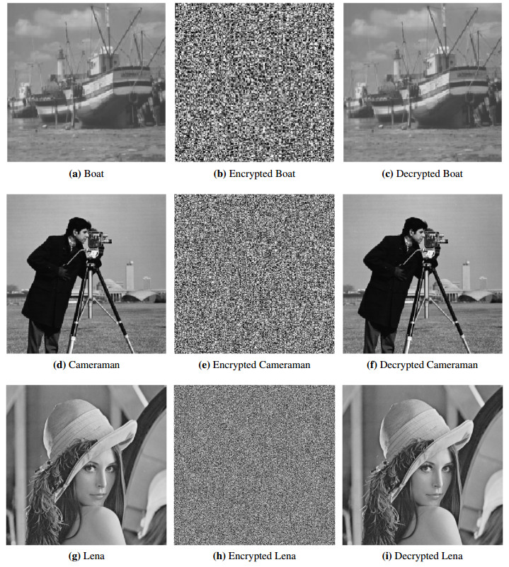
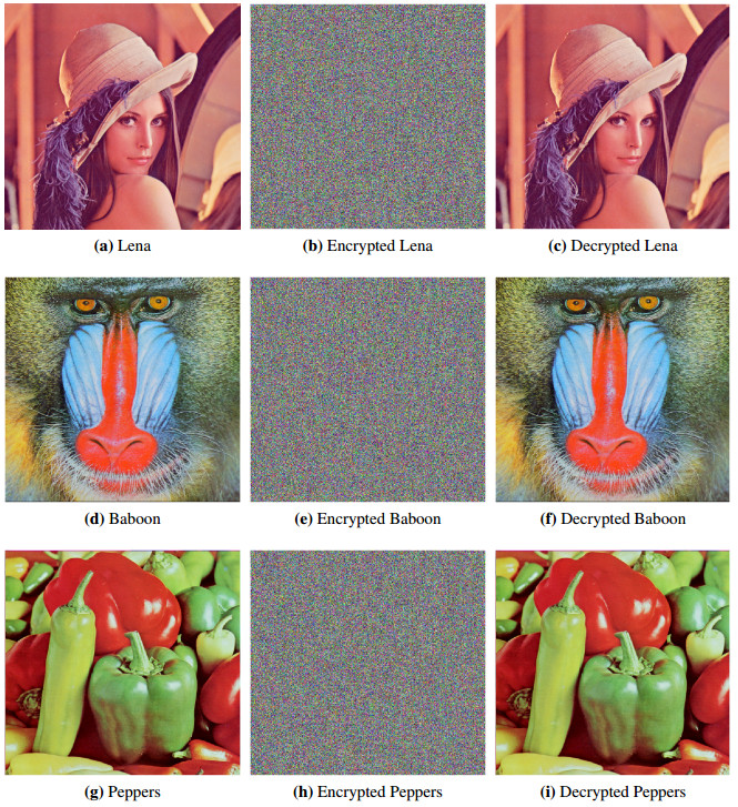
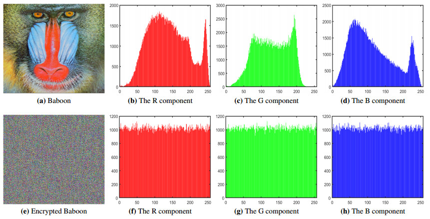
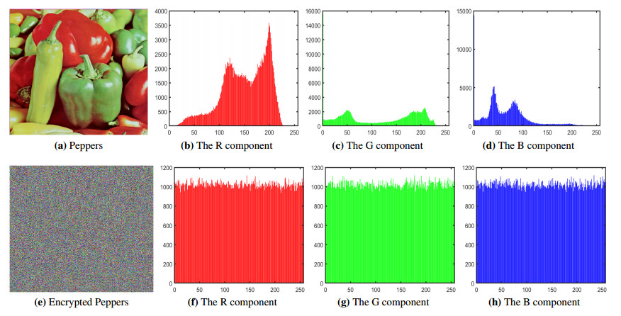
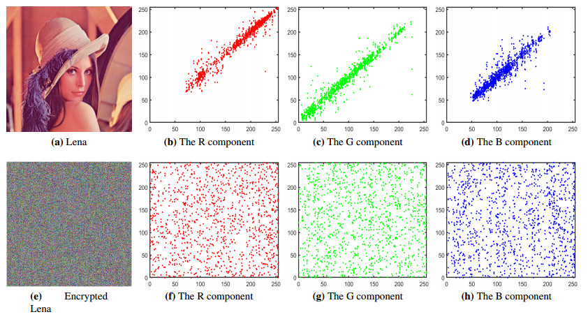
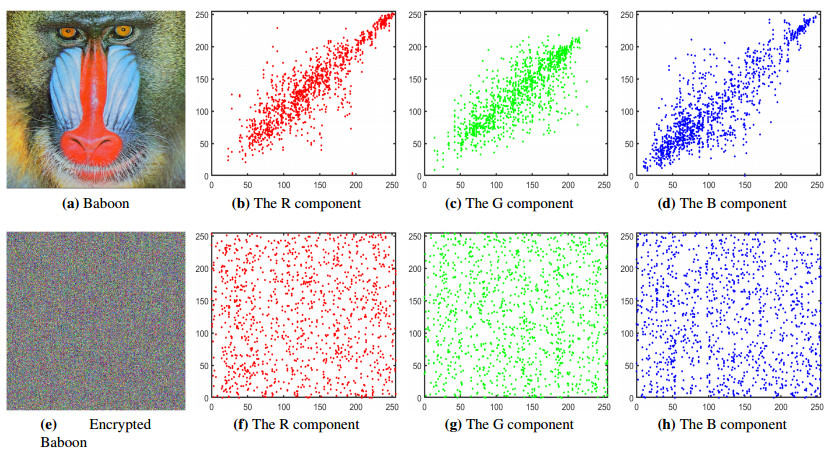
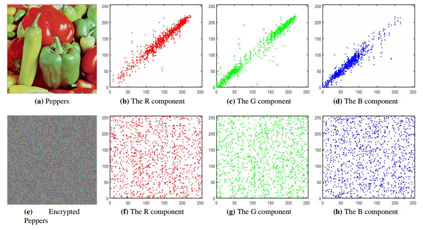
Figure 3 shows the encrypted and decrypted images of Boat (160×160), Cameraman (256×256) and Lena (512×512) in gray format, respectively, Figure 4 shows the encrypted and decrypted images of Lena (512×512), Baboon (512×512) and Peppers (512×512) in RGB format, respectively, we can see that the encrypted image have no features, the original image can be correctly obtained by the decryption algorithm.
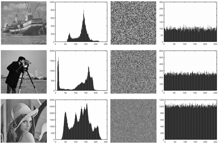
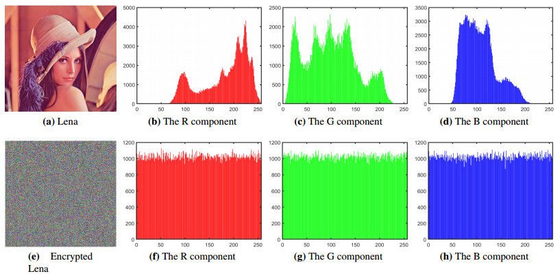
Histogram can intuitively reflect the distribution of each pixel gray, the pixel distribution of original image is generally uneven. Original image has obvious statistical regularity and is often attacked by statistical analysis attacks. For resist this attack, the histogram of the encrypted image must be uniform to disrupt the regularity of the pixels to prevent the attacker to obtain the useful information. Therefore, the histogram distribution of encrypted image more uniform, the encryption algorithm more better, on the contrary, the encryption algorithm is not safe. Figure 5 shows the gray histograms of the Boat, Cameraman and Lena and their encrypted images and decrypted images. Figures 6–8 shows the histograms of the Lena, Baboon and Peppers in R, G, B components. It can be seen from the histogram that the pixels of encrypted image are completely disrupted, the gray values are evenly distributed.
Information entropy is an important index to describe information complexity, the confusion and distribution of encrypted image pixels can be quantified by information entropy.
The value of information entropy more larger, the pixel distribution more uniform and the encryption algorithm more security, on the contrary, the value of information entropy more small, the security more worse. The calculation formula of information entropy H(x) as follows
| H(x)=−255∑i=0P(xi)log2P(xi), |
where xi denotes the grey level and P(xi) is the probability of gray level xi appearing in this image.
In a gray image, there are 256 gray levels, the probability of each gray level is 1/256 for ideal encryption, the information entropy can reach the ideal value 8, when the information entropy is closer to the ideal value 8, the encryption effect is more better. Tables 1 and 2 show the comparison of information entropy results between the proposed encryption algorithm and other encryption algorithms. We can see that the information entropy of the proposed encryption algorithm is very close to the ideal value 8, these show the effectiveness of the proposed encryption algorithm.
| Original image | The proposed encryption algorithm | Ref. [2] | Ref. [4] | Ref. [5] | Ref. [6] | |
| Boat | 6.7252 | 7.9928 | 7.9916 | 7.9890 | 7.9922 | 7.9925 |
| Cameraman | 7.0097 | 7.9974 | 7.9970 | 7.9955 | 7.9973 | 7.9973 |
| Lena | 7.4451 | 7.9992 | 7.9993 | 7.9984 | 7.9993 | 7.9994 |
 DownLoad:
CSV
DownLoad:
CSV
| Original image | The proposed algorithm | Ref. [2] | Ref. [4] | Ref. [5] | Ref. [6] | ||
| Lena | R | 7.2531 | 7.9991 | 7.9993 | 7.9990 | 7.9992 | 7.9993 |
| G | 7.5940 | 7.9991 | 7.9992 | 7.9990 | 7.9991 | 7.9994 | |
| B | 6.9684 | 7.9991 | 7.9992 | 7.9967 | 7.9992 | 7.9993 | |
| Baboon | R | 7.7067 | 7.9992 | 7.9992 | 7.9985 | 7.9991 | 7.9993 |
| G | 7.4744 | 7.9993 | 7.9992 | 7.9981 | 7.9994 | 7.9993 | |
| B | 7.7522 | 7.9992 | 7.9993 | 7.9991 | 7.9993 | 7.9993 | |
| Peppers | R | 7.3388 | 7.9994 | 7.9993 | 7.9983 | 7.9992 | 7.9992 |
| G | 7.4963 | 7.9992 | 7.9993 | 7.9989 | 7.9993 | 7.9993 | |
| B | 7.0583 | 7.9992 | 7.9993 | 7.9990 | 7.9992 | 7.9993 |
DownLoad:
CSV
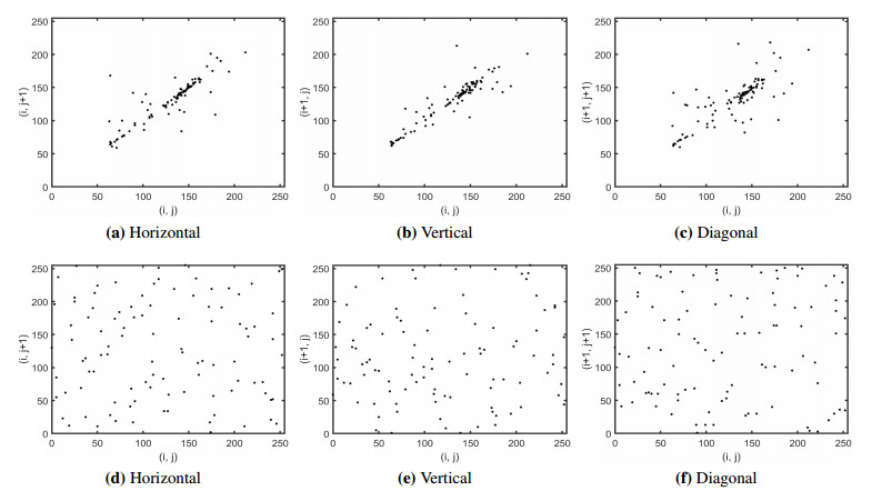
Correlation generally refers to the degree of correlation between two or more pixels. There is a strong correlation between adjacent pixels of the original image. Encryption algorithms must to disrupt these correlated pixels to achieve the desired encryption effect. The adjacent pixel correlation of encrypted image more weak, the encryption effect more better, on the contrary, if the correlation more strong, the encryption effect more bad. The calculation formula of the correlation coefficient Rxy is
| {Rxy=cov(x,y)√D(x)√D(y),D(x)=1MNMN∑i=0(xi−E(x))2,E(x)=1MNMN∑i=0xi,cov(x,y)=1MN(xi−E(x))(yi−E(y)), |
where x and y are the two adjacent pixels, MN is the sum of pixels in the image.
Table 3 shows the correlation coefficients obtained by randomly selecting pixels in the horizontal, vertical and diagonal directions of the original image and encrypted image, where Boat select 100 pixels and Cameraman select 200 pixels. We can see that the correlation coefficients of the encrypted image in all three directions are very close to 0 which show that the encryption algorithm is good to break the correlation of the original pixels. Table 4 is the comparative results of the correlation between different encryption algorithms. In Table 5, we compare the results of Lena in gray and RGB format with other literatures. Observing the results, we can see that most of the correlation coefficient of proposed encryption algorithm are better than Ref.[2,4,5,6].
| Horizontal | Vertical | Diagonal | ||
| Boat | Original image | 9.1129e-01 | 9.1562e-01 | 8.4806e-01 |
| Encrypted image | 4.7347e-04 | 4.7251e-04 | –7.2513e-03 | |
| Cameraman | Original image | 9.3276e-01 | 9.3219e-01 | 9.0618e-01 |
| Encrypted image | 5.0545e-04 | 5.0664e-04 | 2.2202e-03 |
DownLoad:
CSV
| The proposed encryption algorithm | Ref. [2] | Ref. [4] | Ref. [5] | Ref. [6] | ||
| Boat | Horizontal | 4.7347e-04 | –1.0045e-02 | 9.1929e-03 | –4.6696e-03 | –9.1234e-03 |
| Vertical | 4.7251e-04 | –1.0070e-02 | 9.1619e-03 | –4.6957e-03 | –9.1722e-03 | |
| Diagonal | –7.2513e-03 | –1.7840e-03 | –1.1465e-02 | 9.3678e-03 | 1.3823e-02 | |
| Cameraman | Horizontal | 5.0545e-04 | –1.2514e-03 | –3.0978e-03 | 8.1377e-03 | 7.1051e-03 |
| Vertical | 5.0664e-04 | –1.2529e-03 | –3.0955e-03 | 8.1413e-03 | 7.0914e-03 | |
| Diagonal | 2.2202e-03 | 1.1711e-02 | –1.4994e-02 | –4.9900e-03 | –9.2223e-04 |
DownLoad:
CSV
| The proposed encryption algorithm | Ref. [2] | Ref. [4] | Ref. [5] | Ref. [6] | ||
| Gray Lena | 1.6165e-03 | 1.8795e-03 | 4.2927e-03 | 2.0797e-03 | 3.7695e-03 | |
| RGB Lena | R | 1.0036e-03 | 2.2689e-03 | 1.9674e-03 | 1.2921e-03 | 3.6633e-03 |
| G | 1.8628e-03 | 2.5243e-03 | 3.4400e-03 | 2.0831e-03 | 2.4585e-03 | |
| B | 3.7065e-04 | 1.7381e-03 | 2.0731e-03 | 4.7438e-03 | 1.3239e-03 |
DownLoad:
CSV
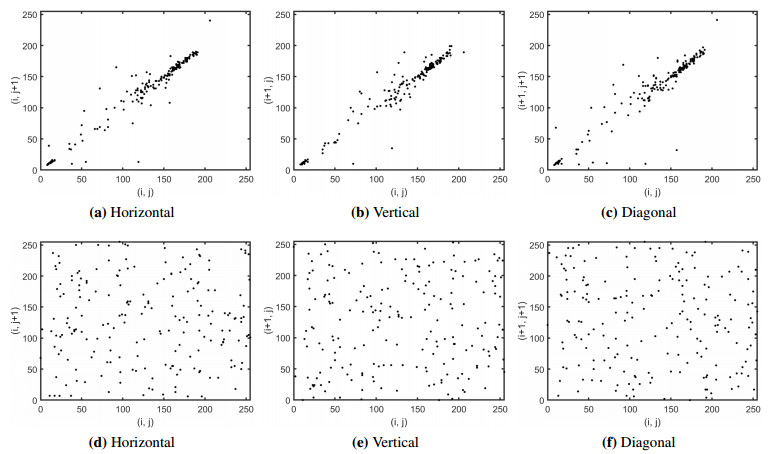
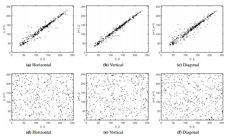
The correlation distribution of the original image and encrypted image in three directions are shown in Figures 9–11. In these graphs, abscissa denotes the pixel value of position (i,j) in this image, ordinate denotes the pixel values of the horizontal adjacent pixel (i,j+1), the vertical adjacent pixel (i+1,j), the diagonal diagonal adjacent pixel (i+1,j+1), respectively. In Figures 12–14, we show scatter distribution of the three directions for the RGB image Lena, Baboon and Peppers, in each component, we draw the scatter plots in three directions together. In histogram of original image, we can see that the correlation between adjacent pixels of the original image is very obvious. Observing the scatter distribution in histogram of encrypted image, we can see that the correlation between the pixels of the encrypted image is completely broken and it has not any rule.
Cipher key sensitivity means that when there is a small change in the key, a completely different encryption effect can be produced. An ideal encryption algorithm should be sensitive to cipher key transformation to ensure the security of the encryption algorithm. There are generally two indicators for evaluating key sensitivity namely number of pixels change rate (NPCR) and unified average changing intensity (UACI), respectively. The calculation formulas are
| {NPCR=M∑i=1N∑j=1D(i,j)MN×100%,D(i,j)={1,C1(i,j)≠C2(i,j),0,otherwise,UACI=1MN×M∑i=1N∑j=1|C1(i,j)−C2(i,j)|255×100%, | (5.1) |
where C1 and C2 are two different encrypted images by use different cipher key. The ideal values of NPCR and UACI are 99.6094% and 33.4635%, respectively. When NPCR and UACI are more closer to the ideal value, the encryption algorithm is more sensitive to the key, the encryption algorithm is more secure. Changing the initial key parameter rmin to rmin+2 to encrypt the Boat and Cameraman, the results of NPCR and UACI are shown in Table 6, we can see that the NPCR and UACI of the proposed encryption algorithm are very close to the ideal value, which indicates that the proposed encryption algorithm is sensitive to the key. In addition, the Table 6 gives the comparison of NPCR and UACI obtained by other encryption algorithms. In Table 7, we show the comparison results of Lena in gray and RGB format, for the Lena in RGB format, we use the average value of each component as the final result of NPCR and UACI.
| The proposed encryption algorithm | Ref. [2] | Ref. [4] | Ref. [5] | Ref. [6] | ||
| Boat | NPCR | 99.625% | 99.629% | 99.668% | 99.586% | 99.590% |
| UACI | 33.345% | 33.281% | 34.515% | 33.595% | 33.472% | |
| Cameraman | NPCR | 99.600% | 99.646% | 99.629% | 99.568% | 99.631% |
| UACI | 32.995% | 33.531% | 33.930% | 33.415% | 33.341% |
DownLoad:
CSV
| The proposed encryption algorithm | Ref. [2] | Ref. [4] | Ref. [5] | Ref. [6] | ||
| Gray Lena | NPCR | 99.606% | 99.601% | 99.582% | 99.570% | 99.593% |
| UACI | 33.448% | 33.352% | 33.870% | 33.428% | 33.466% | |
| RGB Lena | NPCR(AVG) | 99.606% | 99.627% | 99.582% | 99.629% | 99.615% |
| UACI(AVG) | 33.447% | 33.420% | 33.786% | 33.523% | 33.480% |
DownLoad:
CSV
Differential attack is a means for cracking encrypted image, some attackers use the encryption algorithm to encrypt the original image and the changed original image separately to find the relationship between the original image and the encrypted image. Plaintext sensitivity is mainly to test whether the encryption algorithm can resist this differential attack.
We change one pixel value in the original image, then we use the same key to encrypt the original image and the changed image to get two different ciphertext images. We still use the NPCR and UACI index of the formula (5.1) to measure the difference between two encrypted images. In Tables 8 and 9, we arbitrarily changed the original pixels in the position (1, 1), and the results show that the NPCR and UACI is very close to ideal value, which show the reliability of the proposed encryption algorithm. We still use Lena with two formats as an example to show the comparison results of different algorithms, it can be seen that the encryption algorithm in this paper is sensitive to the change of pixels.
| 124→127 | 124→131 | 124→85 | 124→125 | |
| NPCR | 99.602% | 99.684% | 99.629% | 99.687% |
| UACI | 33.972% | 33.440% | 33.591% | 33.784% |
DownLoad:
CSV
| 156→50 | 156→200 | 156→125 | 156→152 | |
| NPCR | 99.657% | 99.605% | 99.605% | 99.577% |
| UACI | 33.428% | 33.562% | 33.416% | 33.324% |
DownLoad:
CSV
| The proposed encryption algorithm | Ref. [2] | Ref. [4] | Ref. [5] | Ref. [6] | ||
| Gray Lena | NPCR | 99.615% | 16.479% | 3.8147e-04% | 99.590% | 99.612% |
| UACI | 33.314% | 5.5649% | 2.9919e-06% | 33.421% | 20.330% | |
| RGB Lena | NPCR(AVG) | 99.621% | 20.391% | 3.8147e-04% | 99.642% | 99.612% |
| UACI(AVG) | 33.577% | 6.8034% | 2.9919e-06% | 33.470% | 20.396% |
DownLoad:
CSV
In Table 11, we compare the results of this paper with the related work in recent years. It can be seen that the effect of the encryption algorithm in this paper can reach the level of the latest research results and has good security.
| H | Horizontal | Vertical | Diagonal | NPCR | UACI | |
| ours | 7.9992 | –1.5041e-03 | –1.5045e-03 | 5.4874e-04 | 99.606% | 33.448% |
| Ref.[2] | 7.9993 | –1.8629e-03 | –1.8619e-03 | 6.1996e-03 | 99.601% | 33.352% |
| Ref.[4] | 7.9984 | 2.6442e-03 | 2.6432e-03 | –9.3217e-04 | 99.582% | 33.870% |
| Ref.[5] | 7.9993 | 1.7772e-03 | 1.7770e-03 | 3.9794e-03 | 99.570% | 33.428% |
| Ref.[6] | 7.9994 | 2.3625e-03 | 2.3609e-03 | 2.0062e-03 | 99.593% | 33.466% |
| Ref.[10] | 7.9923 | 1.158e-03 | 1.98e-04 | –2.26e-04 | 99.594% | 33.381% |
| Ref.[19] | 7.9993 | –2.1e-03 | 2.03e-02 | 8.1e-03 | 99.809% | 33.481% |
| Ref.[38] | 7.7362(AVG) | 1.394e-01 | 3.39e-02 | 7.55e-02 | − | − |
| Ref.[39] | 7.9991 | 2.2e-03 | 1.5e-03 | 2.5e-03 | 99.61% | 33.45% |
| Ref.[13] | 7.9982 | 1.87e-04 | 5.92e-04 | 7.36e-04 | − | − |
| Ref.[9] | 7.9993(AVG) | 1.2233e-02 | 7.6667e-03 | 6.0000e-04 | − | − |
DownLoad:
CSV
Statistical test NIST SP800-22 is widely used to test the randomness of sequences. We use this standard to test the randomness of the binary sequence size of 30 M generated by the proposed algorithm. The 30 binary sequences are generated and each sequence with a size of 106 bits. It can be seen from Table 12 that the binary sequences generated by our algorithm have successfully passed 15 tests. Some information of the test is as follows: the block length M of Block Frequency test is 128, the block length m of Non-Overlapping Template test is 9, the block length m of Overlapping Template test is 9, the block length m of Approximate Entropy test is 10, the block length m of Serial test is 16, the block length M of Linear Complexity test is 500.
| No. | Test name | P-value | Proportion | Result |
| 1 | Frequency | 0.739918 | 29/30 | Success |
| 2 | Block Frequency | 0.602458 | 30/30 | Success |
| 3 | Cumulative Sums | 0.671779 | 29/30 | Success |
| 4 | Runs | 0.299251 | 30/30 | Success |
| 5 | Longest Run | 0.976060 | 30/30 | Success |
| 6 | Rank | 0.299251 | 30/30 | Success |
| 7 | FFT | 0.035174 | 29/30 | Success |
| 8 | Non-Overlapping Template | 0.534146 | 30/30 | Success |
| 9 | Overlapping Template | 0.804337 | 30/30 | Success |
| 10 | Universal | 0.949602 | 30/30 | Success |
| 11 | Approximate Entropy | 0.213309 | 29/30 | Success |
| 12 | Random Excursions | 0.162606 | 17/17 | Success |
| 13 | Random Excursions Variant | 0.162606 | 16/17 | Success |
| 14 | Serial | 0.534146 | 30/30 | Success |
| 15 | Linear Complexity | 0.299251 | 30/30 | Success |
DownLoad:
CSV
The heat flow cryptosystem is an encryption technology that is different from traditional encryption methods. In this paper, the cryptosystem is composed of a nonlinear pseudo-parabolic equation and the barycentric Lagrange interpolation collocation method for solving the equation is proposed. An image encryption algorithm based on the heat flow cryptosystem is designed, the image is divided into different groups and each group performs two diffusions and one scrambling. We give several images with gray and RGB format for simulation experiments, including classical Lena, Baboon and so on. Some common image encryption evaluation indexes are proposed to objectively evaluate the image encryption algorithm, such as histogram, information entropy, correlation key sensitivity, etc. Good experimental results are obtained to support our experiment. The experimental results show that the proposed encryption algorithm performs well in most of the indicators and the encryption algorithm is sensitive to the change of key and plaintext.
Heat flow cryptosystem can also be applied to encryption of text, voice, video and other information. In the future work, we will consider the impact of different types of partial differential equations on the encryption effect and how to improve the time efficiency of the model.
The work of Jin Li was supported by Natural Science Foundation of Hebei Province (Grant No. A2019209533) and National Natural Science Foundation of China (Grant No. 11771398).
The authors declare there is no conflict of interest.
| 1. | Chengye Zou, Yunong Liu, Yongwei Yang, Changjun Zhou, Yang Yu, Yubao Shang, A privacy-preserving license plate encryption scheme based on an improved YOLOv8 image recognition algorithm, 2025, 230, 01651684, 109811, 10.1016/j.sigpro.2024.109811 |

Zhilan Feng, Robert Swihart, Yingfei Yi, Huaiping Zhu. Coexistence in a metapopulation model with explicit local dynamics[J]. Mathematical Biosciences and Engineering, 2004, 1(1): 131-145. doi: 10.3934/mbe.2004.1.131

| Original image | The proposed encryption algorithm | Ref. [2] | Ref. [4] | Ref. [5] | Ref. [6] | |
| Boat | 6.7252 | 7.9928 | 7.9916 | 7.9890 | 7.9922 | 7.9925 |
| Cameraman | 7.0097 | 7.9974 | 7.9970 | 7.9955 | 7.9973 | 7.9973 |
| Lena | 7.4451 | 7.9992 | 7.9993 | 7.9984 | 7.9993 | 7.9994 |
DownLoad:
CSV
| Original image | The proposed algorithm | Ref. [2] | Ref. [4] | Ref. [5] | Ref. [6] | ||
| Lena | R | 7.2531 | 7.9991 | 7.9993 | 7.9990 | 7.9992 | 7.9993 |
| G | 7.5940 | 7.9991 | 7.9992 | 7.9990 | 7.9991 | 7.9994 | |
| B | 6.9684 | 7.9991 | 7.9992 | 7.9967 | 7.9992 | 7.9993 | |
| Baboon | R | 7.7067 | 7.9992 | 7.9992 | 7.9985 | 7.9991 | 7.9993 |
| G | 7.4744 | 7.9993 | 7.9992 | 7.9981 | 7.9994 | 7.9993 | |
| B | 7.7522 | 7.9992 | 7.9993 | 7.9991 | 7.9993 | 7.9993 | |
| Peppers | R | 7.3388 | 7.9994 | 7.9993 | 7.9983 | 7.9992 | 7.9992 |
| G | 7.4963 | 7.9992 | 7.9993 | 7.9989 | 7.9993 | 7.9993 | |
| B | 7.0583 | 7.9992 | 7.9993 | 7.9990 | 7.9992 | 7.9993 |
DownLoad:
CSV
| Horizontal | Vertical | Diagonal | ||
| Boat | Original image | 9.1129e-01 | 9.1562e-01 | 8.4806e-01 |
| Encrypted image | 4.7347e-04 | 4.7251e-04 | –7.2513e-03 | |
| Cameraman | Original image | 9.3276e-01 | 9.3219e-01 | 9.0618e-01 |
| Encrypted image | 5.0545e-04 | 5.0664e-04 | 2.2202e-03 |
DownLoad:
CSV
| The proposed encryption algorithm | Ref. [2] | Ref. [4] | Ref. [5] | Ref. [6] | ||
| Boat | Horizontal | 4.7347e-04 | –1.0045e-02 | 9.1929e-03 | –4.6696e-03 | –9.1234e-03 |
| Vertical | 4.7251e-04 | –1.0070e-02 | 9.1619e-03 | –4.6957e-03 | –9.1722e-03 | |
| Diagonal | –7.2513e-03 | –1.7840e-03 | –1.1465e-02 | 9.3678e-03 | 1.3823e-02 | |
| Cameraman | Horizontal | 5.0545e-04 | –1.2514e-03 | –3.0978e-03 | 8.1377e-03 | 7.1051e-03 |
| Vertical | 5.0664e-04 | –1.2529e-03 | –3.0955e-03 | 8.1413e-03 | 7.0914e-03 | |
| Diagonal | 2.2202e-03 | 1.1711e-02 | –1.4994e-02 | –4.9900e-03 | –9.2223e-04 |
DownLoad:
CSV
| The proposed encryption algorithm | Ref. [2] | Ref. [4] | Ref. [5] | Ref. [6] | ||
| Gray Lena | 1.6165e-03 | 1.8795e-03 | 4.2927e-03 | 2.0797e-03 | 3.7695e-03 | |
| RGB Lena | R | 1.0036e-03 | 2.2689e-03 | 1.9674e-03 | 1.2921e-03 | 3.6633e-03 |
| G | 1.8628e-03 | 2.5243e-03 | 3.4400e-03 | 2.0831e-03 | 2.4585e-03 | |
| B | 3.7065e-04 | 1.7381e-03 | 2.0731e-03 | 4.7438e-03 | 1.3239e-03 |
DownLoad:
CSV
| The proposed encryption algorithm | Ref. [2] | Ref. [4] | Ref. [5] | Ref. [6] | ||
| Boat | NPCR | 99.625% | 99.629% | 99.668% | 99.586% | 99.590% |
| UACI | 33.345% | 33.281% | 34.515% | 33.595% | 33.472% | |
| Cameraman | NPCR | 99.600% | 99.646% | 99.629% | 99.568% | 99.631% |
| UACI | 32.995% | 33.531% | 33.930% | 33.415% | 33.341% |
DownLoad:
CSV
| The proposed encryption algorithm | Ref. [2] | Ref. [4] | Ref. [5] | Ref. [6] | ||
| Gray Lena | NPCR | 99.606% | 99.601% | 99.582% | 99.570% | 99.593% |
| UACI | 33.448% | 33.352% | 33.870% | 33.428% | 33.466% | |
| RGB Lena | NPCR(AVG) | 99.606% | 99.627% | 99.582% | 99.629% | 99.615% |
| UACI(AVG) | 33.447% | 33.420% | 33.786% | 33.523% | 33.480% |
DownLoad:
CSV
| 124→127 | 124→131 | 124→85 | 124→125 | |
| NPCR | 99.602% | 99.684% | 99.629% | 99.687% |
| UACI | 33.972% | 33.440% | 33.591% | 33.784% |
DownLoad:
CSV
| 156→50 | 156→200 | 156→125 | 156→152 | |
| NPCR | 99.657% | 99.605% | 99.605% | 99.577% |
| UACI | 33.428% | 33.562% | 33.416% | 33.324% |
DownLoad:
CSV
| The proposed encryption algorithm | Ref. [2] | Ref. [4] | Ref. [5] | Ref. [6] | ||
| Gray Lena | NPCR | 99.615% | 16.479% | 3.8147e-04% | 99.590% | 99.612% |
| UACI | 33.314% | 5.5649% | 2.9919e-06% | 33.421% | 20.330% | |
| RGB Lena | NPCR(AVG) | 99.621% | 20.391% | 3.8147e-04% | 99.642% | 99.612% |
| UACI(AVG) | 33.577% | 6.8034% | 2.9919e-06% | 33.470% | 20.396% |
DownLoad:
CSV
| H | Horizontal | Vertical | Diagonal | NPCR | UACI | |
| ours | 7.9992 | –1.5041e-03 | –1.5045e-03 | 5.4874e-04 | 99.606% | 33.448% |
| Ref.[2] | 7.9993 | –1.8629e-03 | –1.8619e-03 | 6.1996e-03 | 99.601% | 33.352% |
| Ref.[4] | 7.9984 | 2.6442e-03 | 2.6432e-03 | –9.3217e-04 | 99.582% | 33.870% |
| Ref.[5] | 7.9993 | 1.7772e-03 | 1.7770e-03 | 3.9794e-03 | 99.570% | 33.428% |
| Ref.[6] | 7.9994 | 2.3625e-03 | 2.3609e-03 | 2.0062e-03 | 99.593% | 33.466% |
| Ref.[10] | 7.9923 | 1.158e-03 | 1.98e-04 | –2.26e-04 | 99.594% | 33.381% |
| Ref.[19] | 7.9993 | –2.1e-03 | 2.03e-02 | 8.1e-03 | 99.809% | 33.481% |
| Ref.[38] | 7.7362(AVG) | 1.394e-01 | 3.39e-02 | 7.55e-02 | − | − |
| Ref.[39] | 7.9991 | 2.2e-03 | 1.5e-03 | 2.5e-03 | 99.61% | 33.45% |
| Ref.[13] | 7.9982 | 1.87e-04 | 5.92e-04 | 7.36e-04 | − | − |
| Ref.[9] | 7.9993(AVG) | 1.2233e-02 | 7.6667e-03 | 6.0000e-04 | − | − |
DownLoad:
CSV
| No. | Test name | P-value | Proportion | Result |
| 1 | Frequency | 0.739918 | 29/30 | Success |
| 2 | Block Frequency | 0.602458 | 30/30 | Success |
| 3 | Cumulative Sums | 0.671779 | 29/30 | Success |
| 4 | Runs | 0.299251 | 30/30 | Success |
| 5 | Longest Run | 0.976060 | 30/30 | Success |
| 6 | Rank | 0.299251 | 30/30 | Success |
| 7 | FFT | 0.035174 | 29/30 | Success |
| 8 | Non-Overlapping Template | 0.534146 | 30/30 | Success |
| 9 | Overlapping Template | 0.804337 | 30/30 | Success |
| 10 | Universal | 0.949602 | 30/30 | Success |
| 11 | Approximate Entropy | 0.213309 | 29/30 | Success |
| 12 | Random Excursions | 0.162606 | 17/17 | Success |
| 13 | Random Excursions Variant | 0.162606 | 16/17 | Success |
| 14 | Serial | 0.534146 | 30/30 | Success |
| 15 | Linear Complexity | 0.299251 | 30/30 | Success |
DownLoad:
CSV
| Original image | The proposed encryption algorithm | Ref. [2] | Ref. [4] | Ref. [5] | Ref. [6] | |
| Boat | 6.7252 | 7.9928 | 7.9916 | 7.9890 | 7.9922 | 7.9925 |
| Cameraman | 7.0097 | 7.9974 | 7.9970 | 7.9955 | 7.9973 | 7.9973 |
| Lena | 7.4451 | 7.9992 | 7.9993 | 7.9984 | 7.9993 | 7.9994 |
| Original image | The proposed algorithm | Ref. [2] | Ref. [4] | Ref. [5] | Ref. [6] | ||
| Lena | R | 7.2531 | 7.9991 | 7.9993 | 7.9990 | 7.9992 | 7.9993 |
| G | 7.5940 | 7.9991 | 7.9992 | 7.9990 | 7.9991 | 7.9994 | |
| B | 6.9684 | 7.9991 | 7.9992 | 7.9967 | 7.9992 | 7.9993 | |
| Baboon | R | 7.7067 | 7.9992 | 7.9992 | 7.9985 | 7.9991 | 7.9993 |
| G | 7.4744 | 7.9993 | 7.9992 | 7.9981 | 7.9994 | 7.9993 | |
| B | 7.7522 | 7.9992 | 7.9993 | 7.9991 | 7.9993 | 7.9993 | |
| Peppers | R | 7.3388 | 7.9994 | 7.9993 | 7.9983 | 7.9992 | 7.9992 |
| G | 7.4963 | 7.9992 | 7.9993 | 7.9989 | 7.9993 | 7.9993 | |
| B | 7.0583 | 7.9992 | 7.9993 | 7.9990 | 7.9992 | 7.9993 |
| Horizontal | Vertical | Diagonal | ||
| Boat | Original image | 9.1129e-01 | 9.1562e-01 | 8.4806e-01 |
| Encrypted image | 4.7347e-04 | 4.7251e-04 | –7.2513e-03 | |
| Cameraman | Original image | 9.3276e-01 | 9.3219e-01 | 9.0618e-01 |
| Encrypted image | 5.0545e-04 | 5.0664e-04 | 2.2202e-03 |
| The proposed encryption algorithm | Ref. [2] | Ref. [4] | Ref. [5] | Ref. [6] | ||
| Boat | Horizontal | 4.7347e-04 | –1.0045e-02 | 9.1929e-03 | –4.6696e-03 | –9.1234e-03 |
| Vertical | 4.7251e-04 | –1.0070e-02 | 9.1619e-03 | –4.6957e-03 | –9.1722e-03 | |
| Diagonal | –7.2513e-03 | –1.7840e-03 | –1.1465e-02 | 9.3678e-03 | 1.3823e-02 | |
| Cameraman | Horizontal | 5.0545e-04 | –1.2514e-03 | –3.0978e-03 | 8.1377e-03 | 7.1051e-03 |
| Vertical | 5.0664e-04 | –1.2529e-03 | –3.0955e-03 | 8.1413e-03 | 7.0914e-03 | |
| Diagonal | 2.2202e-03 | 1.1711e-02 | –1.4994e-02 | –4.9900e-03 | –9.2223e-04 |
| The proposed encryption algorithm | Ref. [2] | Ref. [4] | Ref. [5] | Ref. [6] | ||
| Gray Lena | 1.6165e-03 | 1.8795e-03 | 4.2927e-03 | 2.0797e-03 | 3.7695e-03 | |
| RGB Lena | R | 1.0036e-03 | 2.2689e-03 | 1.9674e-03 | 1.2921e-03 | 3.6633e-03 |
| G | 1.8628e-03 | 2.5243e-03 | 3.4400e-03 | 2.0831e-03 | 2.4585e-03 | |
| B | 3.7065e-04 | 1.7381e-03 | 2.0731e-03 | 4.7438e-03 | 1.3239e-03 |
| The proposed encryption algorithm | Ref. [2] | Ref. [4] | Ref. [5] | Ref. [6] | ||
| Boat | NPCR | 99.625% | 99.629% | 99.668% | 99.586% | 99.590% |
| UACI | 33.345% | 33.281% | 34.515% | 33.595% | 33.472% | |
| Cameraman | NPCR | 99.600% | 99.646% | 99.629% | 99.568% | 99.631% |
| UACI | 32.995% | 33.531% | 33.930% | 33.415% | 33.341% |
| The proposed encryption algorithm | Ref. [2] | Ref. [4] | Ref. [5] | Ref. [6] | ||
| Gray Lena | NPCR | 99.606% | 99.601% | 99.582% | 99.570% | 99.593% |
| UACI | 33.448% | 33.352% | 33.870% | 33.428% | 33.466% | |
| RGB Lena | NPCR(AVG) | 99.606% | 99.627% | 99.582% | 99.629% | 99.615% |
| UACI(AVG) | 33.447% | 33.420% | 33.786% | 33.523% | 33.480% |
| 124→127 | 124→131 | 124→85 | 124→125 | |
| NPCR | 99.602% | 99.684% | 99.629% | 99.687% |
| UACI | 33.972% | 33.440% | 33.591% | 33.784% |
| 156→50 | 156→200 | 156→125 | 156→152 | |
| NPCR | 99.657% | 99.605% | 99.605% | 99.577% |
| UACI | 33.428% | 33.562% | 33.416% | 33.324% |
| The proposed encryption algorithm | Ref. [2] | Ref. [4] | Ref. [5] | Ref. [6] | ||
| Gray Lena | NPCR | 99.615% | 16.479% | 3.8147e-04% | 99.590% | 99.612% |
| UACI | 33.314% | 5.5649% | 2.9919e-06% | 33.421% | 20.330% | |
| RGB Lena | NPCR(AVG) | 99.621% | 20.391% | 3.8147e-04% | 99.642% | 99.612% |
| UACI(AVG) | 33.577% | 6.8034% | 2.9919e-06% | 33.470% | 20.396% |
| H | Horizontal | Vertical | Diagonal | NPCR | UACI | |
| ours | 7.9992 | –1.5041e-03 | –1.5045e-03 | 5.4874e-04 | 99.606% | 33.448% |
| Ref.[2] | 7.9993 | –1.8629e-03 | –1.8619e-03 | 6.1996e-03 | 99.601% | 33.352% |
| Ref.[4] | 7.9984 | 2.6442e-03 | 2.6432e-03 | –9.3217e-04 | 99.582% | 33.870% |
| Ref.[5] | 7.9993 | 1.7772e-03 | 1.7770e-03 | 3.9794e-03 | 99.570% | 33.428% |
| Ref.[6] | 7.9994 | 2.3625e-03 | 2.3609e-03 | 2.0062e-03 | 99.593% | 33.466% |
| Ref.[10] | 7.9923 | 1.158e-03 | 1.98e-04 | –2.26e-04 | 99.594% | 33.381% |
| Ref.[19] | 7.9993 | –2.1e-03 | 2.03e-02 | 8.1e-03 | 99.809% | 33.481% |
| Ref.[38] | 7.7362(AVG) | 1.394e-01 | 3.39e-02 | 7.55e-02 | − | − |
| Ref.[39] | 7.9991 | 2.2e-03 | 1.5e-03 | 2.5e-03 | 99.61% | 33.45% |
| Ref.[13] | 7.9982 | 1.87e-04 | 5.92e-04 | 7.36e-04 | − | − |
| Ref.[9] | 7.9993(AVG) | 1.2233e-02 | 7.6667e-03 | 6.0000e-04 | − | − |
| No. | Test name | P-value | Proportion | Result |
| 1 | Frequency | 0.739918 | 29/30 | Success |
| 2 | Block Frequency | 0.602458 | 30/30 | Success |
| 3 | Cumulative Sums | 0.671779 | 29/30 | Success |
| 4 | Runs | 0.299251 | 30/30 | Success |
| 5 | Longest Run | 0.976060 | 30/30 | Success |
| 6 | Rank | 0.299251 | 30/30 | Success |
| 7 | FFT | 0.035174 | 29/30 | Success |
| 8 | Non-Overlapping Template | 0.534146 | 30/30 | Success |
| 9 | Overlapping Template | 0.804337 | 30/30 | Success |
| 10 | Universal | 0.949602 | 30/30 | Success |
| 11 | Approximate Entropy | 0.213309 | 29/30 | Success |
| 12 | Random Excursions | 0.162606 | 17/17 | Success |
| 13 | Random Excursions Variant | 0.162606 | 16/17 | Success |
| 14 | Serial | 0.534146 | 30/30 | Success |
| 15 | Linear Complexity | 0.299251 | 30/30 | Success |
